In this post, we introduce a training strategy that addresses vanishing gradients in quantum neural networks (QNNs), and makes better use of the resources provided by noisy intermediate-scale quantum (NISQ) devices. This is a short summary of the paper "Layerwise learning for quantum neural networks", which is joint work by the Volkswagen Machine Learning Research Lab (Patrick van der Smagt), the Data:Lab (Andrea Skolik, Martin Leib), and Google AI Quantum (Jarrod R. McClean, Masoud Mohseni).

Quantum neural networks

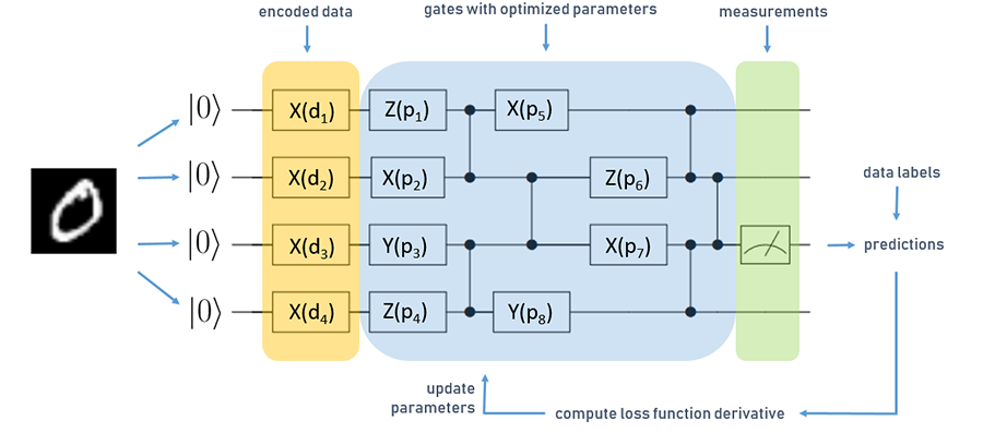
Training a QNN is not that much different from training a classical neural network, just that instead of optimising network weights, we optimise the parameters of a quantum circuit. A quantum circuit looks like this:

Fig. 1: Simplified QNN for a classification task with four qubits

The circuit is read from left to right, and each horizontal line corresponds to one qubit in the register of the quantum computer, each initialised in the zero state. The boxes denote parametrised operations (or “gates”) on qubits which are executed sequentially.

In this case we have three different types of operations, X, Y, and Z. Vertical lines denote two-qubit gates, which can be used to generate entanglement in the QNN—one of the resources that lets quantum computers outperform their classical counterparts. We denote one layer as one operation on each qubit, followed by a sequence of gates that connect pairs of qubits to generate entanglement.

The figure above shows a simplified QNN for learning classification of MNIST digits. First, we have to encode the data set into quantum states. We do this by using a data encoding layer, marked orange in the figure above. In this case, we transform our input data into a vector, and use the vector values as parameters d for the data encoding layers’ operations. Based on this input, we execute the part of the circuit marked in blue, which represents the trainable gates of our QNN, denoted by p.

The last operation in the quantum circuit is a measurement. During computation, the quantum device performs operations on superpositions of classical bitstrings. When we perform a readout on the circuit, the superposition state collapses to one classical bitstring, which is the output of the computation that we get. The so-called collapse of the quantum state is probabilistic, to get a deterministic outcome we average over multiple measurement outcomes.

In the above picture, marked in green, we perform measurements on the third qubit and use these to predict labels for our MNIST examples. We compare this to the true data label and compute gradients of a loss function just as in a classical neural network. These types of QNNs are called “hybrid quantum-classical”, as the parameter optimisation is handled by a classical computer; in our case, we used the Adam optimiser.

Vanishing gradients, aka barren plateaus

It turns out that QNNs also suffer from vanishing gradients, just like classical neural networks. Since the reason for vanishing gradients in QNNs is fundamentally different from classical NNs (where they are also called "saddle points"), a new term has been adopted for them: barren plateaus. Covering all details of this important phenomenon is out of the scope of this post, so we refer the interested reader to the paper that first introduced barren plateaus in QNN training landscapes or this tutorial on barren plateaus on the TenforFlow Quantum site for a hands-on example.

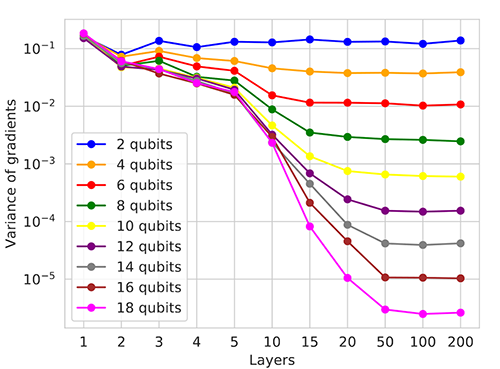
In short, barren plateaus occur when quantum circuits are initialszed randomly—in the circuit illustrated above this means picking operations and their parameters at random. This is a fundamental problem for training parametrised quantum circuits, and gets worse as the number of qubits and the number of layers in a circuit grows, as we can see in the figure below.

Fig. 2: Variance of gradients decays as a function of the number of qubits and layers in a random circuit

For the algorithm we introduce below, the key thing to understand here is that the more layers we add to a circuit, the smaller the variance in gradients will get. On the other hand, similarly to classical NNs, the QNN’s representational capacity also increases with its depth. The problem here is that in addition, the optimisation landscape flattens in many places as we increase the circuit’s size, so it gets harder to find even a local minimum.

Remember that for QNNs, outputs are estimated from taking the average over a number of measurements. The smaller the quantity we want to estimate, the more measurements we will need to get an accurate result. If these quantities are much smaller compared to the effects caused by measurement uncertainty or hardware noise, they can't be reliably determined and the circuit optimisation will basically turn into a random walk.

To successfully train a QNN, we have to avoid random initialisation of the parameters, and also have to stop the QNN from randomising during training as its gradients get smaller, for example when it approaches a local minimum. For this, we can either limit the architecture of the QNN (e.g., by picking certain gate configurations, which requires tuning the architecture to the task at hand), or control the updates to parameters such that they won’t become random.

Layerwise learning

In our paper Layerwise learning for quantum neural networks we introduce an approach to avoid initialisation on a plateau as well as the network ending up on a plateau during training.

Let’s look at an example of layerwise learning (LL) in action, on the learning task of binary classification of MNIST digits. First, we need to define the structure of the layers we want to stack. As we make no assumptions about the learning task at hand, we choose the same layout for our layers as in the figure above: one layer consists of random gates on each qubit initialised with zero, and two-qubit gates which connect qubits to enable generation of entanglement.

We designate a number of start layers, in this case only one, which will always stay active during training, and specify the number of epochs to train each set of layers. Two other hyperparameters are the number of new layers we add in each step, and the number of layers that are maximally trained at once. Here we choose a configuration where we add two layers in each step, and freeze the parameters of all previous layers, except the start layer, such that we only train three layers in each step. We train each set of layers for 10 epochs, and repeat this procedure ten times until our circuit consists of 21 layers overall. By doing this, we use the fact that shallow circuits produce larger gradients compared to deeper ones, and with this avoid initialising on a plateau.

This provides us with a good starting point in the optimisation landscape to continue training larger contiguous sets of layers. As another hyperparameter, we define the percentage of layers we train together in the second phase of the algorithm. Here, we choose to split the circuit in half, and alternatingly train both parts, where the parameters of the inactive parts are always frozen. We call one training sequence where all partitions have been trained once a sweep, and we perform sweeps over this circuit until the loss converges. When the full set of parameters is always trained—call it “complete-depth learning” (CDL)—one bad update step can affect the whole circuit and lead it into a random configuration and therefore a barren plateau, from which it cannot escape.

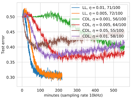
Let’s compare our training strategy to CDL, which is one of the standard techniques used to train QNNs. To get a fair comparison, we use exactly the same circuit architecture as the one generated by the LL strategy before, but now update all parameters simultaneously in each step. To give CDL a chance to train, we initialise the parameters with zero instead of randomly. As we don’t have access to a real quantum computer yet, we simulate the probabilistic outputs of the QNN, and choose a relatively low value for the number of measurements that we use to estimate each prediction the QNN makes—which is 10 in this case. Assuming a 10kHZ sampling rate on a real quantum computer, we can estimate the experimental wall-clock time of our training runs as shown below:

Fig. 3: Comparison of layerwise- and complete depth learning with different learning rates η. We trained 100 circuits for each configuration, and averaged over those that achieved a final test error lower than 0.5 (number of succeeding runs in legend).

With this small number of measurements, we can investigate the effects of the different gradient magnitudes of the LL and CDL approaches: if gradient values are larger, we get more information out of 10 measurements than for smaller values. The less information we have to perform our parameter updates, the higher the variance in the loss, and the risk to perform an erroneous update that will randomise the updated parameters and lead the QNN onto a plateau. This variance can be lowered by choosing a smaller learning rate, so we compare LL and CDL strategies with different learning rates in the figure above.

Notably, the test error of CDL runs increases with the runtime, which might look like overfitting at first. However, each curve in this figure is averaged over many runs, and what is actually happening here is that more and more CDL runs randomise during training, unable to recover. In the legend we show that a much larger fraction of LL runs achieved a classification error on the test set lower than 0.5 compared to CDL, and also did it in less time.

In summary, layerwise learning increases the probability of successfully training a QNN with overall better generalisation error in less training time, which is especially valuable on NISQ devices. For more details on the implementation and theory of layerwise learning, please refer to the full paper. We also released a notebook with an implementation of layerwise learning in TensorFlow Quantum, which can be found in TFQ research repository.

arXiv