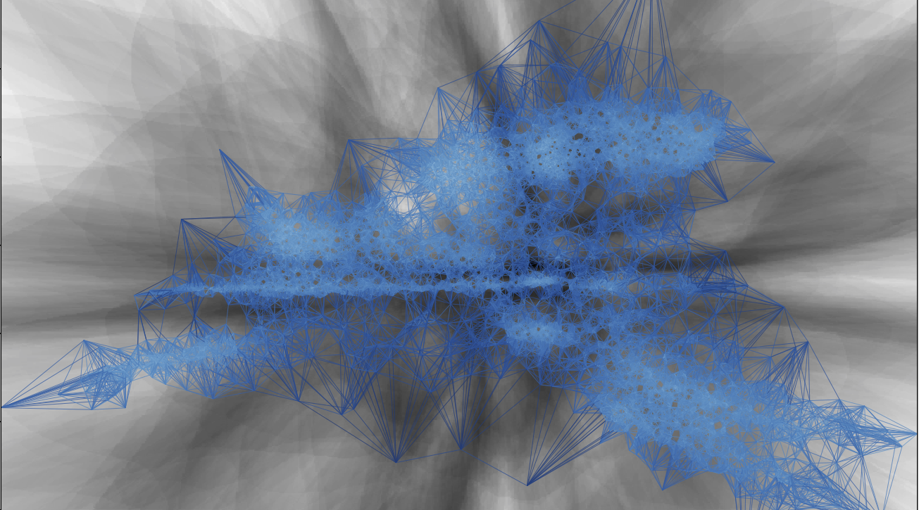
Neural samplers such as variational autoencoders (VAEs) or generative adversarial networks (GANs) approximate distributions by transforming samples from a simple random source—the latent space—to a more complex distribution—corresponding to the distribution from which is data is sampled.

Typically, the data set is sparse, while the latent space is compact. Consequently, points that are separated by low-density regions in observation space will be pushed together in latent space, and the spaces get distored. In effect, stationary distances in the latent space are poor proxies for similarity in the observation space. How can this be solved?

We transfer ideas from Riemannian geometry to this setting, letting the distance between two points be the shortest path on a Riemannian manifold induced by the transformation. The method yields a principled distance measure, provides a tool for visual inspection of deep generative models, and an alternative to linear interpolation in latent space.

Riemannian geometry for generative models

Our model is based on the importance-weighted autoencoder (IWAE), but can be used for any generative model. In the IWAE, the observable data \(\mathbf{x} \in \mathbb{R}^{N_{x}}\) are represented through latent variables \(\mathbf{z} \in \mathbb{R}^{N_{z}}\), that are based on hidden characteristics in \(\mathbf{x}\).

A Riemannian space is a differentiable manifold \(M\) with an additional metric to describe its geometric properties. This enables assigning an inner product in the tangent space at each point \(\mathbf{z}\) in the latent space through the corresponding metric tensor \(\mathbf{G} \in \mathbb{R}^{N_z \times N_z}\), i.e.,

with \(\mathbf{z}' \in T_{\mathbf{z}}M\) and \(\mathbf{z} \in M\). \(T_{\mathbf{z}}M\) is the tangent space.

Treating the latent space of a VAE as a Riemannian manifold allows us to compute the observation space distance of latent variables. Assuming we have a trajectory \(\gamma:[0, 1]\rightarrow\mathbb{R}^{N_{z}}\) in the Riemannian (latent) space that is transformed by a continuous function \(f(\gamma(t))\) (decoder) to an \(N_{x}\)-dimensional Euclidean (observation) space. The length of this trajectory in the observation space, referred to as the Riemannian distance, is defined by

with \(\dot{\gamma}(t)\) denoting the time-derivative of the trajectory. \(\sqrt{\big<\gamma'(t), \gamma'(t)\big>_{\gamma(t)}}\) is the Riemannian velocity \(\phi(t)\).

The metric tensor is defined as \(\mathbf{G}=\mathbf{J}^{T}\mathbf{J}\), with \(\mathbf{J}\) as the Jacobian of the decoder. The trajectory which minimises the Riemannian distance \(L(\gamma)\) is referred to as the shortest path geodesic. We integrate the metric tensor with \(n\) equidistantly spaced sampling points along \(\gamma\) to approximate the distance, i.e.,

We use the magnification factor (MF) to show the sensitivity of the generative models in 2D latent space and evaluate the approximated geodesic. The \(\text{MF}(\mathbf{z})\equiv \sqrt{\det\mathbf{G}(\mathbf{z})}\) can be interpreted as the scaling factor when moving from the Riemannian (latent) to the Euclidean (observation) space, due to the change of variables.

Approximate geodesics

We proposed two approaches to approximate geodesics—neural network-based and graph-based approaches.

Neural network-based geodesics

As written in Chen et al. (2018), we use a neural network \(g_{\omega}:\mathbb{R} \rightarrow \mathbb{R}^{N_{z}}\) to approximate the curve \(\gamma\) in the latent space, where \(\omega\) are the weights and biases.

With the start and end points of the curve in the latent space given as \(\mathbf{z}_0\) and \(\mathbf{z}_1\), we consider the following constrained optimisation problem:

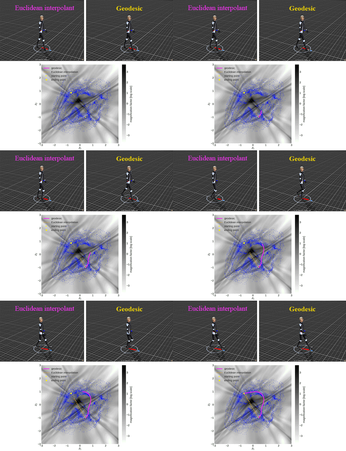
There is an example of showing the difference between the geodesic and Euclidean interpolant using CMU human motion dataset:

Graph-based geodesics

There are several challenges of the NN-based or similar (e.g., ODE) approaches:

• it needs the second derivative of the decoder during the optimisation process;
• it scales poorly with the dimensionality of the observable and the latent space;
• computing the second derivative limits the selection of the neural network’s activation function.

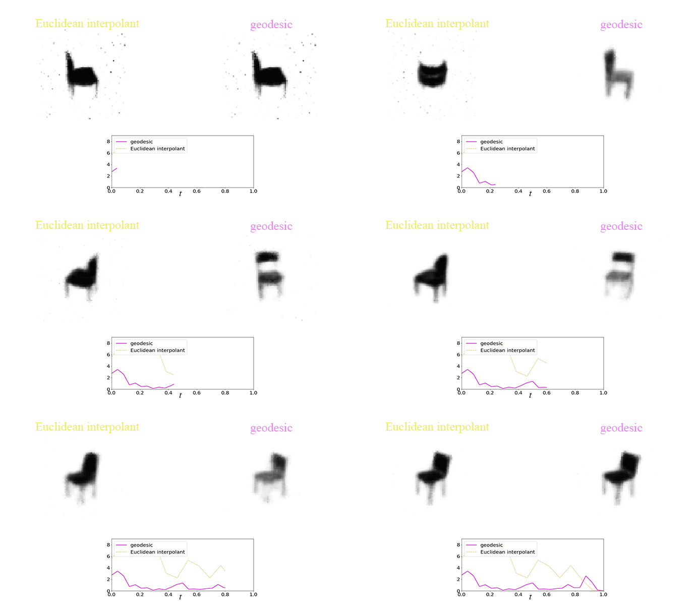
To bypass these hurdles we introduce a graph-based approach Chen et al. (2019), where a discrete and finite graph is built in the latent space using a binary tree data structure, a k-d tree, with edge weights based on Riemannian distances. Once the graph has been built, geodesics can be approximated by applying a classic search algorithm, \(\mathrm{A}^\star\).

Building the graph.

The graph is structured as a k-d tree, a special case of binary space partitioning trees, where each leaf node corresponds to a k-dimensional vector. The nodes of the graph are obtained by encoding the observable data \(\mathbf{X} = \{ \mathbf{x}^{(1)},\dots,\mathbf{x}^{(N)} \}\) into their latent representations \(\mathbf{z}^{(i)}\). This is done by using the respective mean values of the approximate posterior \(q_{\phi}(\mathbf{z}^{(i)}|\mathbf{x}^{(i)})\). Each node is connected by an undirected edge to its k-nearest neighbours. The edge weights are set to Riemannian distances \(L(\gamma)\), where \(\gamma\) is the straight line between the related pair of nodes.

Approximating geodesics.

A classic graph-traversing method to obtain the shortest path between nodes is \(\mathrm{A}^\star\) search. It is an iterative algorithm that, given a graph \(\mathcal{G}\), maintains a sorted list of nodes that can be visited in the current state. The list is typically initialised with the starting node and is being sorted according to the estimated cost of including node \(n\) into the optimal path. The estimated cost is computed by \(f(n) = g(n) + h(n),\) where \(g(n)\) is the cost of the path from the starting node \(n_\mathrm{start}\) to \(n\) and \(h(n)\) is a heuristic function that estimates the remaining cost from \(n\) to the target node \(n_\mathrm{target}\).

There is an example of showing the difference between the geodesic and Euclidean interpolant using the chair dataset:

Applied to robot active learning

Our method is applied to robot motion generation and active learning. See more details in Chen et al. (2018).

Bibliography

Nutan Chen, Francesco Ferroni, Alexej Klushyn, Alexandros Paraschos, Justin Bayer, and Patrick van der Smagt. Fast approximate geodesics for deep generative models. In ICANN. 2019. URL: https://arxiv.org/abs/1812.08284. ↩
Nutan Chen, Alexej Klushyn, Richard Kurle, Xueyan Jiang, Justin Bayer, and Patrick van der Smagt. Metrics for deep generative models. In AISTATS, 1540–1550. 2018. URL: https://arxiv.org/abs/1711.01204. ↩
Nutan Chen, Alexej Klushyn, Alexandros Paraschos, Djalel Benbouzid, and Patrick van der Smagt. Active learning based on data uncertainty and model sensitivity. IEEE/RSJ IROS, 2018. URL: https://arxiv.org/abs/1808.02026. ↩