Intuition and experience. Probably, that's the answer you would get if you happen to ask deep learning engineers how they chose the hyperparameters of a neural network. Depending on their familiarity with the problem, they might have done some good three to five full dataset runs until a satisfactory result popped up. Now, you might say, we surely could automate this, right, after all we do it implicitly in our heads? Well, yes, we definitely could, but should we?

Imagine you want to search among a single hyperparameter, say the depth of the network. How about some \(\{3, 5, 8, 11\}\)-layer deep networks. This will require you at least four training cycles consisting in creation, initialisation, training until convergence and evaluation on a held-out test set. Maybe that's not that bad. What happens, however, if you decide to search for an optimal layer size too? In convolutional neural networks, you can even pick strides, filter sizes and so on. The search space quickly grows beyond any imaginable human patience. And let's admit it, most of the time you just pretend to be happy with what you end up with after a couple of trials.

Nevertheless, the situation is far from hopeless as there's still a way to learn the architecture directly from the data! In the following blog post we will look into that and show an approach that allows us to probabilistically interpret the learnt architecture and thereby spot engineered design misspecifications. Moreover, we will do it the Bayesian way, meaning that we will incorporate our architectural views merely as prior beliefs rather than hard constraints.

Bayesian deep learning

Being Bayesian about anything as complex as a neural architecture is all but easy. In essence, we are asking for the form of a posterior distribution over some parameters \(\alpha\) after observing labelled data \((\mathbf{x},\, \mathbf{y})\), or \(p\left(\alpha\mid\mathbf{x},\, \mathbf{y}\right)\) for short. The Bayes' rule of probability tells us that:

Due to the intractability of computing the evidence \(p\left(\mathbf{y}\mid\mathbf{x}\right)\) we don't even dream of estimating \(p\left(\alpha\mid\mathbf{x},\, \mathbf{y}\right)\) exactly. Instead we will reside to approximate inference techniques such as variational Bayes (VB) where we approximate \(p\left(\alpha\mid\mathbf{x},\, \mathbf{y}\right)\) with a \(\theta\)-parameterised distribution \(q_\theta\left(\alpha\mid\mathbf{x},\, \mathbf{y}\right)\). Fortunately, Jordan et al. (1999) showed that the dissimilarity between \(q_\theta\left(\alpha\mid\mathbf{x},\, \mathbf{y}\right)\) and \(p\left(\alpha\mid\mathbf{x},\, \mathbf{y}\right)\) can be decreased without explicitly computing \(p\left(\mathbf{y}\mid\mathbf{x}\right)\). The trick is to learn the \(\theta\) such that a quantity called the Evidence Lower BOund is maximised:

However, this too is not computable in closed form and we will have to approximate it with sampling. We can go on and on discussing the issues and merits of this approach but we will stop here and instead go straight into the core of this post—applying VB to efficiently infer an approximate posterior distribution over the architectural parameters.

Bayesian architecture learning

We can think of certain structural hyperparameters as discrete random variables, e.g. the depth of a network and the size of a layer are well described by positive integer numbers. A categorical distribution may seem like a good modelling choice as it is flexible enough to represent every discrete distribution with domain \(\{1, 2, \dots, K\}\)—only thing we have to do is to learn the probabilities \(\boldsymbol{\pi} = (\pi_1, \pi_2, \dots, \pi_K)\) for each category. Unfortunately, to do this we cannot use the backpropagation algorithm because a sample of the categorical distribution is a non-differentiable transformation of \(\boldsymbol{\pi}\) and some external noise \(\boldsymbol{\epsilon}\):

Instead we use a continuous approximation to it due to Maddison et al. (2016) and Jang et al. (2016), where the non-differentiable \({\mathrm{arg}\,\mathrm{max}}\) operator is replaced with the smooth \(\mathrm{softmax}\):

Notice that \(\mathbf{\tilde{c}} = (\tilde{c}_1, \tilde{c}_2, \dots, \tilde{c}_K)\) is not a one-hot vector anymore and that the temperature parameter \(\tau\) controls the degree of discreteness. But, most importantly, we can express, say, the size of the layer as a sample of a distribution the parameters of which we can learn via backpropagation!

In order to bridge the gap between this result and the \(\mathcal{L}_{\text{ELBO}}\) objective we discussed earlier, we only have to define a prior distribution over the architectural variable and express the data likelihood as a function of it without breaking the differentiability of the neural network. But that's just nothing compared to the mental and computational effort needed to find an optimal architecture using a search-based procedure. So let's do it quickly.

Adaptive layer size

Let \(\alpha\) be the random variable representing the number of units within a layer. We can define prior and approximate posterior distributions respectively as:

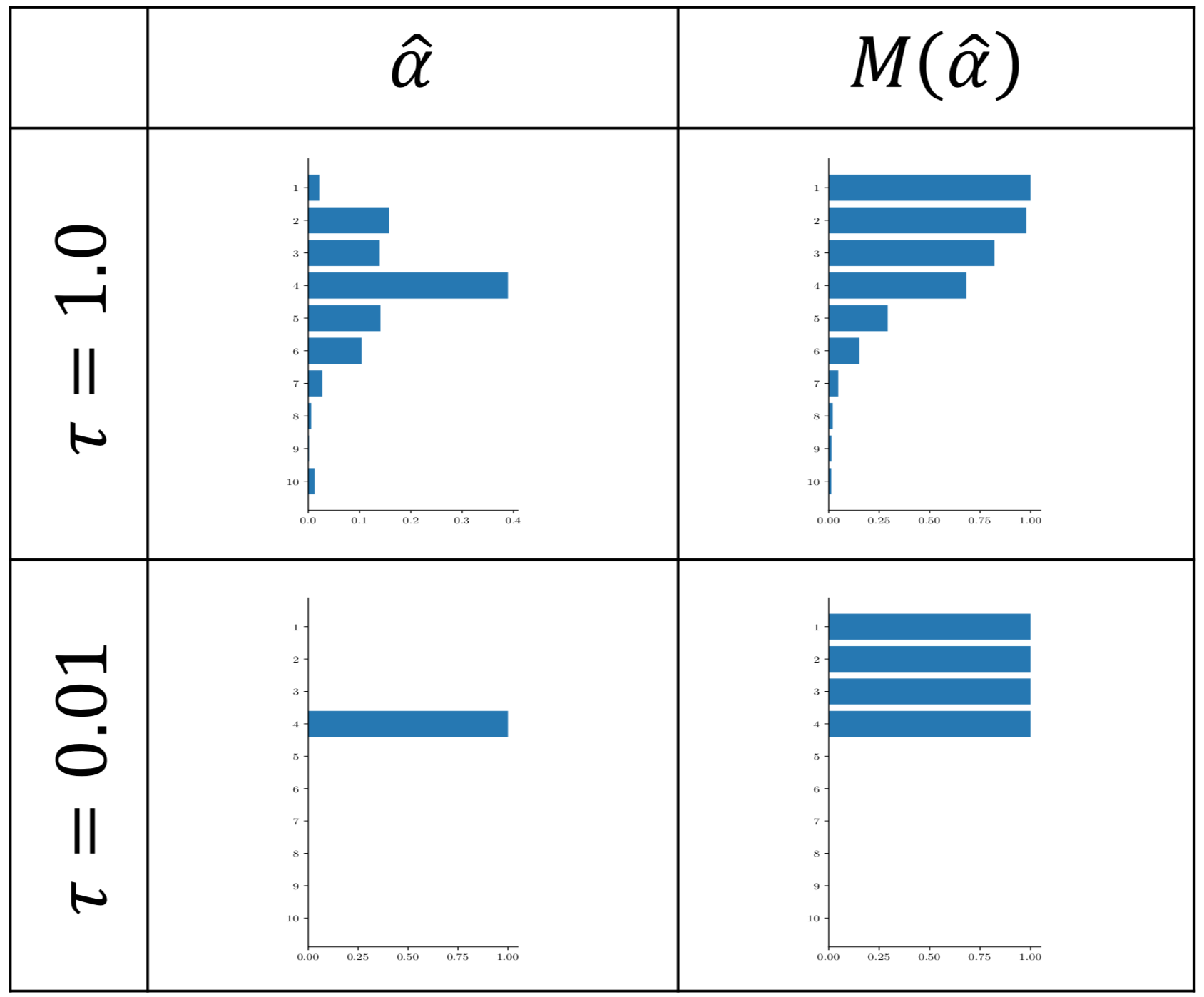
where we fix \(\tau\) and learn only \(\boldsymbol{\pi}\) to facilitate our task. If we want to learn the layer size for example, we must express the output of a layer as a deterministic operation of the sample \(\hat{\alpha} \sim q_{\boldsymbol{\pi}, \tau}(\alpha\mid\mathbf{x}, \mathbf{y})\) and the weights and biases of it. One way to do it is to deterministically compute a quasi-binary mask \(M(\hat{\alpha})\) that (approximately) lets \({\mathrm{arg}\,\mathrm{max}}_i \hat{\alpha}_i\) unit activations through and shadows the rest, e.g. we can build it as a linear combination with coefficients \(\hat{\alpha}\) of some cleverly-chosen set of binary masks:

Below you can see a concrete sample in the left and the corresponding mask in the right. The sharpness of this mask is mainly determined by \(\tau\) but keep in mind that the gradients are inversely proportional to \(\tau\) and learning becomes instable for \(\tau \rightarrow 0\).

Job done, let's see what we can learn with it... well, wait a second. Before we move on, we remark that the variational parameters \(\boldsymbol{\pi}\) are so unconstrained that it might be hard to interpret the posterior distribution. What would be the desired size in a multi-modal scenario? How do we read out the uncertainty over the layer size? After all, at the end of the day we would like to be able to tailor the architecture according to the learnt posterior distribution and fix it for good. To do this, we will have to constrain \(\boldsymbol{\pi}\) in a way that ensures unimodality and an easily interpretable variance. We reside to the (modified) chicken soup of the distributions—the truncated Normal distribution. That is, instead of \(\boldsymbol{\pi}\) we now learn \(\mu\) and \(\sigma\) and set:

We can simply read out \(\mu\) to get the most likely estimate for the size of the layer and \(\sigma\) (which is not a standard deviation any more!) can be interpreted as an uncertainty around that point.

Adaptive network depth

To model the total depth of a network we can't just broadcast the mask over the outputs of each layer, as even a single fully masked intermediate layer will kill the output of the network. We go about this by using trainable skip connections which allow to bypass redundant layers. We can implement them by representing the layer as a convex combination of its input \(\mathbf{x}\) and output \(f(\mathbf{W}\mathbf{x} + \mathbf{b})\) controlled by a stochastic mixing coefficient \(\gamma \sim \mathrm{ConcreteBernoulli(\pi)}\):

In other words, we let \(\pi\) represent the probability of skipping a layer and we learn it via backpropagation pretty much the same way we did for the adaptive layer size. Naturally, we can also define a concrete Bernoulli prior \(p_{\pi_\text{prior}}(\gamma)\). Without further ado, let's look into an example!

Case-study: regression

There is hardly any more trivial and yet intuitive way to see how neural networks work, than fitting a nicely plottable one-dimensional noisy data. In order to show the effectiveness of the methods we will consider two cases. First, we will show the adaptive layer size applied on a single layer neural network with 50 units and then we will go deep with a rather "narrow" 10-layer network.

Finding the optimal layer size

For the sake of insightfulness we will put a rather silly architectural prior distribution with \(\mu_\text{prior}=1\) and \(\sigma_\text{prior}=2\) and hope that the network will learn a minimalistic layer architecture that also explains the data well. In the leftmost figure you can see the training data and the current best fit, computed by sampling from \(q_{\boldsymbol{\pi}, \tau}(\alpha\mid\mathbf{x}, \mathbf{y})\). The middle plot shows the truncated normal distribution from which \(\boldsymbol{\pi}\) is derived and the rightmost image is an alternative visualisation showing the full history from the initialisation to the final solution.

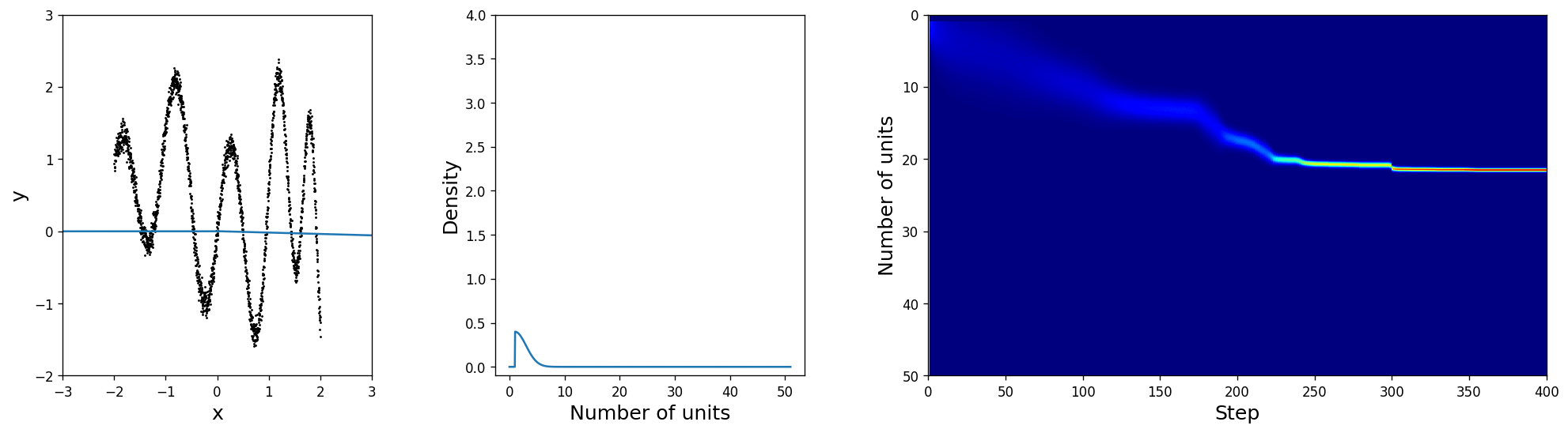
Indeed, the posterior over the size, as shown in the middle, shifts towards something more reasonable and thus unlocks more and more of the layer's capacity. It is only a matter of time for \(\mu\) to settle and \(\sigma\) to shrink at the nearly optimal unit count. Also, notice how the uncertainty is larger in the beginning when the layer size is inadequate and gradually sharpens later on, which gives us a good insight into how well the network structure is suited for the problem even without looking at the predictions!

Finding the optimal network depth

Ok, so far so good. We have shown that we can fit the data with one hidden layer hosting at least 21 units. To see whether we can also learn the depth of a deeper network, we will initialise 10 hidden layers of 5 units each, with a \(\pi_\text{prior} = 0.99\) (i.e. we skip a layer with 99% probability). Obviously the task cannot be reliably solved by a single layer, so the network will have to learn to overcome the rather strong prior. The animation below shows the fit on the left and the probabilities \(\pi\) for each layer, colour-coded in shades of grey where black means definitively "skip" and white "let through" respectively.

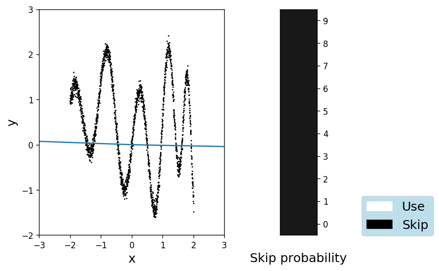
It is interesting to see how the network quickly learns to use the heavily muted layers, while gradually unlocking more and more of them. Apparently 5 layers of 5 units are enough to explain the data and the posterior over the skip variable \(q_\pi(\gamma)\) remains pretty close to the prior for the remaining 5 layers.

If we wish, we could also combine the adaptive layer size and network depth approaches in a single elastic network and learn all hyperparameters jointly. For now, we leave this as an exercise for you!

Final words

In this blog post we have seen that it is very much possible to learn the basic architecture of feed-forward densely connected neural networks while in the same time tuning their weights to explain the data. This comes handy when you have no clue how to configure your model and also don't have the time and computational power to explore large hyperparameter spaces over many runs. Keep in mind that we have shown a method to infer an optimal layer size for standard layer types but there is no conceptual difficulty in extending it to convolutional and recurrent layers, where the mask is applied over the channels and the time steps axis respectively. Finally, we remark that despite its convenience, this technique adds an additional layer of complexity to the model. It is therefore best to use it only as a tool to infer near-optimal architectures. Once found, please do initialise a rigid model accordingly and train it until convergence.

Good luck!

This work was published at the International Conference on Artificial Intelligence and Statistics (AISTATS) 2019

Bibliography

Eric Jang, Shixiang Gu, and Ben Poole. Categorical reparameterization with gumbel-softmax. arXiv preprint arXiv:1611.01144, 2016. ↩
Michael I Jordan, Zoubin Ghahramani, Tommi S Jaakkola, and Lawrence K Saul. An introduction to variational methods for graphical models. Machine learning, 37(2):183–233, 1999. ↩
Chris J Maddison, Andriy Mnih, and Yee Whye Teh. The concrete distribution: a continuous relaxation of discrete random variables. arXiv preprint arXiv:1611.00712, 2016. ↩