Machine-learning algorithms thrive in environments where data is abundant. In the land of scarce data, blessed are those who have simulators. The recent successes in Go or Atari games would be much harder to achieve without the ability to parallelise millions of perfect game simulations.

But in many other domains, we cannot use this approach. For instance robotics, where simulations often fall short. After all, only phenomena that are understood well enough can be simulated. Everything else is necessarily idealised and abstracted. If we had accurate simulators for such domains, we could devise much more efficient learning algorithms around them. Just like we don't need to play millions of real-world games to make a machine learn Go, we wouldn't need to run dozens of robots for countless hours to acquire sufficient data.

The key to simulators in these domains is accurate prediction. As Niels Bohr pointedly put it: "Prediction is very difficult, especially if it's about the future." Luckily, machine learning is not alone in its quest for better predictions. Better predictions are the driving factor behind many scientific disciplines: any scientific hypothesis must allow falsifiable predictions.

In this post, we will be looking into the approaches developed in other fields. We will draw inspirations from established methods, and introduce our own algorithm Deep Variational Bayes Filters (DVBF, Karl et al. (2017)). DVBF solves shortcomings of many established method with the help of machine learning.

Differential equations

Let's start in Niels Bohr's own domain, physics. For 350 years, physicists have been using an elegant way for describing processes—differential equations. At its core, a differential equation is a predictor: how will a process evolve over time? And does that prediction comply with the observations we make in the real world?

Why are differential equations such a successful tool? Let us look at a simple example, a one-link robot, also known as damped pendulum. We try to predict the displacement angle \(\theta\) over time. This process is governed by the differential equation

This simple example highlights the core features of differential equations at work.

1. The differential equation is compact and local: we prefer to know the changes that will happen in a short horizon instead of the brittle global evolution. Instead of specifying a complicated, often brittle function \(\theta(t, \theta_0)\) for the angle at any point in time \(t\) from any initial displacement \(\theta_0\), it describes how the angle acceleration \(\ddot\theta\) is affected by the current state of the system, its displacement angle \(\theta\) and the angle velocity \(\dot\theta\).
2. Because we locally look at the pendulum, we achieve a modular description: the differential equation consists of two separate terms—damping from friction, \(\frac bm\dot\theta\), and acceleration from gravity, \(\frac gL \sin\theta\). In a global description, we would need to consider their complex interplay. The local description makes things simpler, and it allows us to add or leave away assumptions.

State-space systems

Now we know the differential equation governing the pendulum. It depends on angle and angle velocity, and given these we can predict the evolution of the process. Great! What's left?

Well, we need to obtain angle and angle velocity starting configuration for our prediction. The easy way out is to mount appropriate sensors and to keep our fingers crossed someone calibrated them properly. But more often than not, this is not an option. Plus it's boring! A camera, instead, is relatively cheap and easy to install.

On the right is a (synthetic) video sequence of a simulated pendulum. In fact, for a human it's easy to predict how this video sequence will continue, because we have understood the underlying physical process. But how do we access the information about the state of the pendulum that is hidden in the pixels? Let us rephrase the question: how does the video frame at time \(t\) differ from angle and angle velocity at that point in time? What makes it easier to describe the dynamical process in terms of angles and angle velocities rather than pixels?

Answering this question lead to the concept of state-space systems. In these systems, we make a distinction between the latent state \(\mathbf z_t\) of a system, like angle and velocity, and observations \(\mathbf x_t\) of it, like video frames. A state-space system consists of two components:

1. Dynamics on the state, like a differential equation (or, because we siletnly switched to the more computer-friendly discrete systems, a difference equation). It is a low-dimensional, often minimal description of the process. We will generally refer to this as the (latent) state transition.
2. A rendering or measurement process that yields observations based on the latent state. This can mean that the latent state is only partially observable. We will refer to this process as the emission model.

The core idea is that the true state is not observed, hence latent state. We can only infer it from the observations: what is the state, given the observations we have made? This sounds a lot like posterior inference! Let's look at state-space systems from a statistical perspective.

Filtering

The simple latent process then becomes a distribution over a sequence of latent states, \(p(\mathbf z_{1:T})\). Likewise, the emission process is a distribution over the observations given the latent states, \(p(\mathbf x_{1:T}\mid\mathbf z_{1:T})\). Our question—what is the state, given the observations we have made?—can now be answered in a rigorous framework. The answer is the posterior distribution \(p(\mathbf z_{1:T}\mid\mathbf x_{1:T})\), and by Bayes' theorem \(p(\mathbf z_{1:T}\mid\mathbf x_{1:T}) \propto p(\mathbf x_{1:T}\mid\mathbf z_{1:T})p(\mathbf z_{1:T})\). In our scenarios, this posterior distribution is also called filter distribution: it filters the quintessential information, the latent state, from the observations. The resulting algorithms are called Bayes filters.

Arguably the most famous implementation of such a Bayes filter is the Kalman filter. Airplane autopilots depend on its tracking abilities, as does your GPS navigation system, and many, many more.

Where is the limit?

Done!? Not quite yet. The Kalman filter succeeds by putting strong assumptions on the state-space system, in that both the difference equation and the measurement process need to be linear Gaussian models. The Kalman filter is provably optimal in that setting. These assumptions are (approximately) valid in many interesting scenarios. The Kalman filter is the go-to algorithm for tracking because large-scale natural motions are approximately linear and Gaussian. After all, it's safe to board an airplane with a Kalman filter position tracking.

Yet, highly nonlinear observations, like camera frames, cannot be filtered by Kalman filters. In general cases, the Bayes filter is intractable. And there is an even bigger caveat: in all the stages so far, we assumed that we know the underlying process, the difference equation, and through Bayes' formula the filter depends on it. But coming up with suitable state space representations is laborious, costly, and requires a significant amount of domain knowledge.

Deep Variational Bayes Filters

Luckily, over the past years machine learning has taken a deep dive into unsupervised representation learning. The most useful tool for our purposes is inference via amortised variational Bayes. It was popularised by variational auto-encoders (VAE, Kingma and Welling (2014)).

A VAE learns a model \(p(\mathbf x \mid \mathbf z)\) with a fixed prior \(p(\mathbf z)\), and simultaneously an approximate posterior \(q(\mathbf z \mid \mathbf x)\). The conditional random variables are implemented with neural networks. If we extend this idea to sequential data, we can tackle both caveats: we can learn an approximate Bayes filter even for nonlinear data; simultaneously, we learn the state transition in latent space plus the emission model. Both leverage the modelling powers of neural networks to overcome the shortcomings of methods like the Kalman filter.

This is the core idea behind Deep Variational Bayes Filters (DVBF): We overcome the limitations of well-understood Bayes filters, and we do so by surgically replacing limiting components with neural networks. Instead of entirely replacing a well-established approach, we extend it to previously intractable data with findings from deep learning. This gives us the best of both worlds.

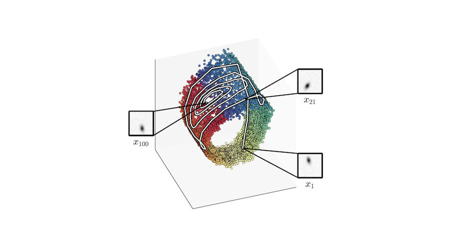
And here is how DVBF looks in action on the pendulum example:

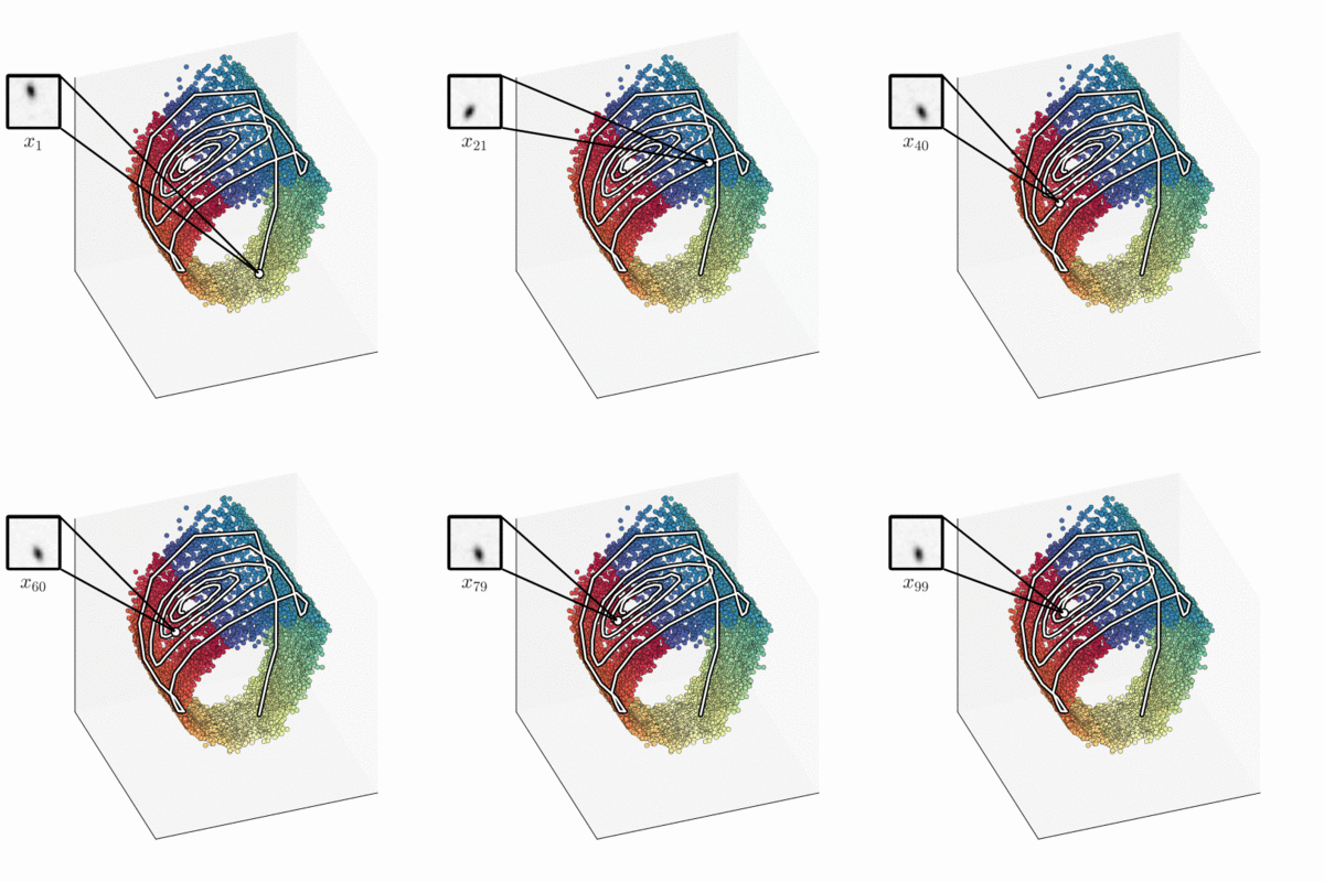
The approximate filter distribution, implemented by a neural net, maps the sequence of frames into a three-dimensional latent space. The model has learnt that a two-dimensional barrel-shaped manifold is a good state-space representation.

Intriguingly, when we compare the latent state to the ground truth, we find a strong relation. Without a notion of pendulum physics or even angles, the learning algorithm autonomously encodes the real-world angle on a circle, and the ground-truth angle velocity is encoded perpendicular to that. The smooth colouring using ground-truth angle data highlights that.

At this point, our journey in this article has gone full circle: we started off by looking at the differential equation of the pendulum, and after a series of further considerations, we have found an unsupervised algorithm that learns transitions akin to this very differential equation from raw data.

And just like differential equations, this approach is compact, local, and modular. Especially the modularity can be used to our advantage. Instead of using a less interpretable neural network, we may use other components that make use of some system knowledge. We can compose the latent state process from simple principles, rather than ever more complex models in the observation space.

We've also trained a probabilistic model of our system. A simulator! We can sample the behaviour of the system without interacting with it in the real world.

What's next?

Arguably, we dealt with not more than an illustrative example in this post. Yet applications of DVBF all but stop here. Having an explicit model for sequence data is very valuable, and we will close this post by looking at two advanced applications.

The first successful application of DVBF is Empowerment Karl et al. (2019). Loosely speaking, empowerment is a measure of how diversely and effectively an agent can influence its environment. As such, it is a natural candidate for intrinsic motivation in control an reinforcement learning. We have shown that Empowerment can lead to meaningful behaviour in very different agents and environments in the absence of any other cost function.

At the core of our Empowerment algorithm is DVBF. An agent needs to be aware of the consequences of its actions to be able to estimate its current Empowerment. If the agent can query a simulation rather than interacting with the environment, this stabilises the empowerment estimates.

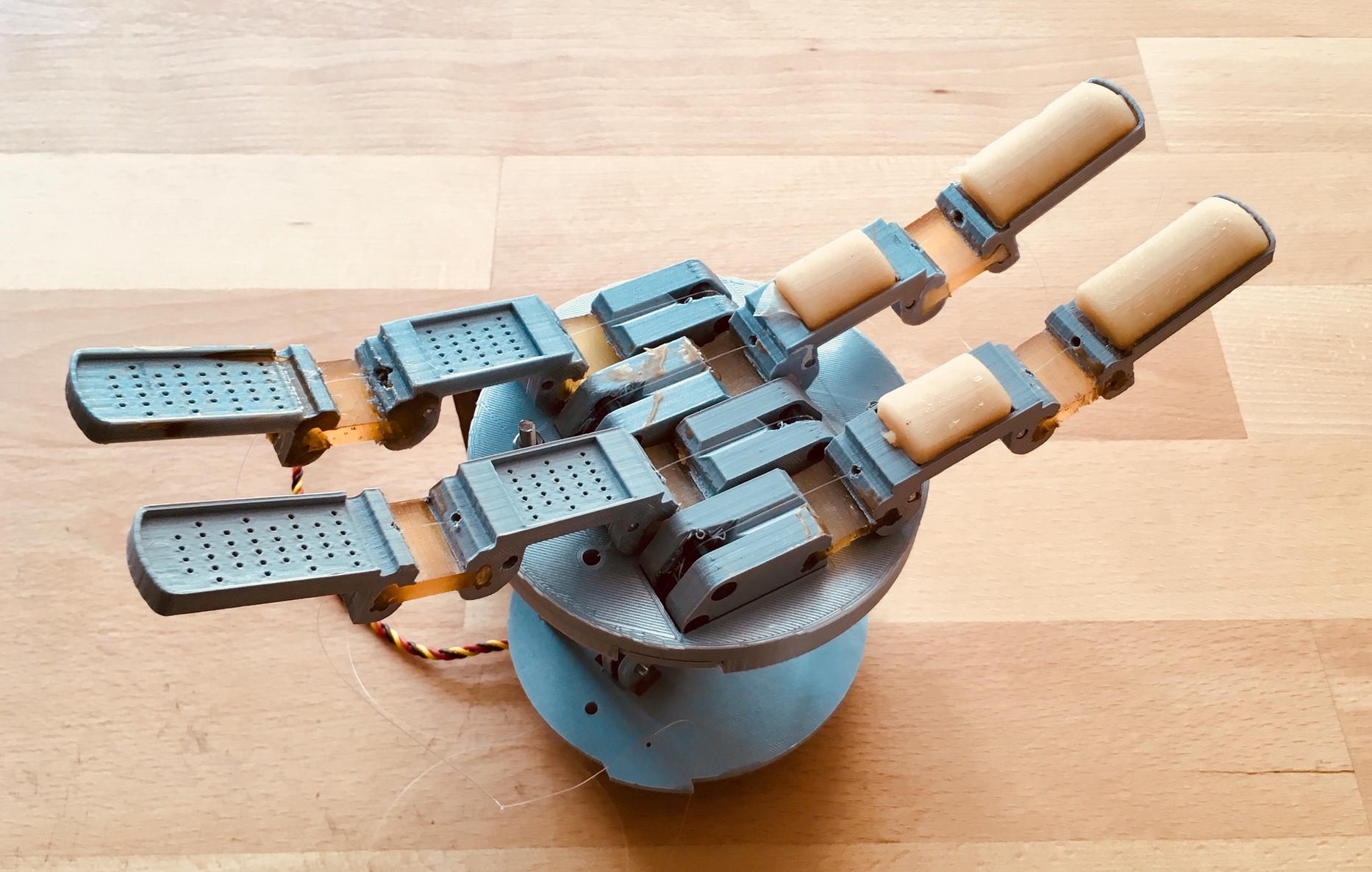
Another important application is a new view on sensors. Sensors are expensive because it is difficult to manufacture them with good calibration properties. In our lab, we have applied this principle to artificial skin. Rather than the costly state-of-the-art sensors, we can produce durable tactile sensors at a fraction of the cost, and reach sensor accuracy by post-processing the low-quality data with DVBF.

We will take a closer look at these two cases in later posts on this blog.

An open-source version of DVBF is available here.

arXiv

Bibliography

Maximilian Karl, Maximilian Soelch, Justin Bayer, and Patrick van der Smagt. Deep variational Bayes filters: unsupervised learning of state space models from raw data. In Proceedings of the International Conference on Learning Representations (ICLR). 2017. URL: http://arxiv.org/abs/1605.06432. ↩
Maximilian Karl, Maximilian Soelch, Philip Becker-Ehmck, Djalel Benbouzid, Patrick van der Smagt, and Justin Bayer. Unsupervised real-time control through variational empowerment. In International Symposium on Robotics Research (ISRR). 2019. URL: http://arxiv.org/abs/1710.05101, arXiv:1710.05101. ↩
Diederik P Kingma and Max Welling. Auto-encoding variational Bayes. In Proceedings of the 2nd International Conference on Learning Representations (ICLR). 2014. ↩