Variational autoencoders (VAEs) (Kingma and Welling, 2013), (Rezende et al., 2014) are a class of probabilistic latent-variable models for unsupervised learning and one of the models we base our work on. The idea behind the VAE is that the learned probabilistic model and the corresponding (approximate) posterior distribution of the latent variables provide a decoder/encoder pair that can capture semantically meaningful features of the data.

In this blog post, we address the issue of learning informative latent representations/encodings. In classifiable data, this may be representations that cluster according to some discrete features of the data. In regression data, important variations in data should be aligned with the axes of the latent space.

The latent representation in a VAE is strongly influenced by the prior on those latent variables. In the vanilla VAE, this prior is a standard normal distribution. This can be a limiting factor because it leads to over-regularising the posterior distribution, resulting in latent representations that do not represent well the structure of the data (Alemi et al., 2018). Several methods have been proposed to alleviate this problem, including:

• using specialised optimisation algorithms that try to find local/global minima of the training objective that correspond to informative latent representations (Bowman et al., 2016), (Sonderby et al., 2016), (Higgins et al., 2017), (Rezende and Viola, 2018);
• or defining and learning complex prior distributions that can better model the encoded data manifold (Chen et al., 2016), (Tomczak and Welling, 2018).

In the following, we will introduce a combination of these two approaches.

Background: Variational Autoencoders

VAEs are a class of unsupervised learning methods, where we assume that the data \(\mathbf{x}\in \mathbb{R}^n\) is generated by the probabilistic model

and the data \(\mathcal{D} = \{\mathbf{x}_i\}_{i=1}^N\) is a set of identically distributed and independently generated data points.

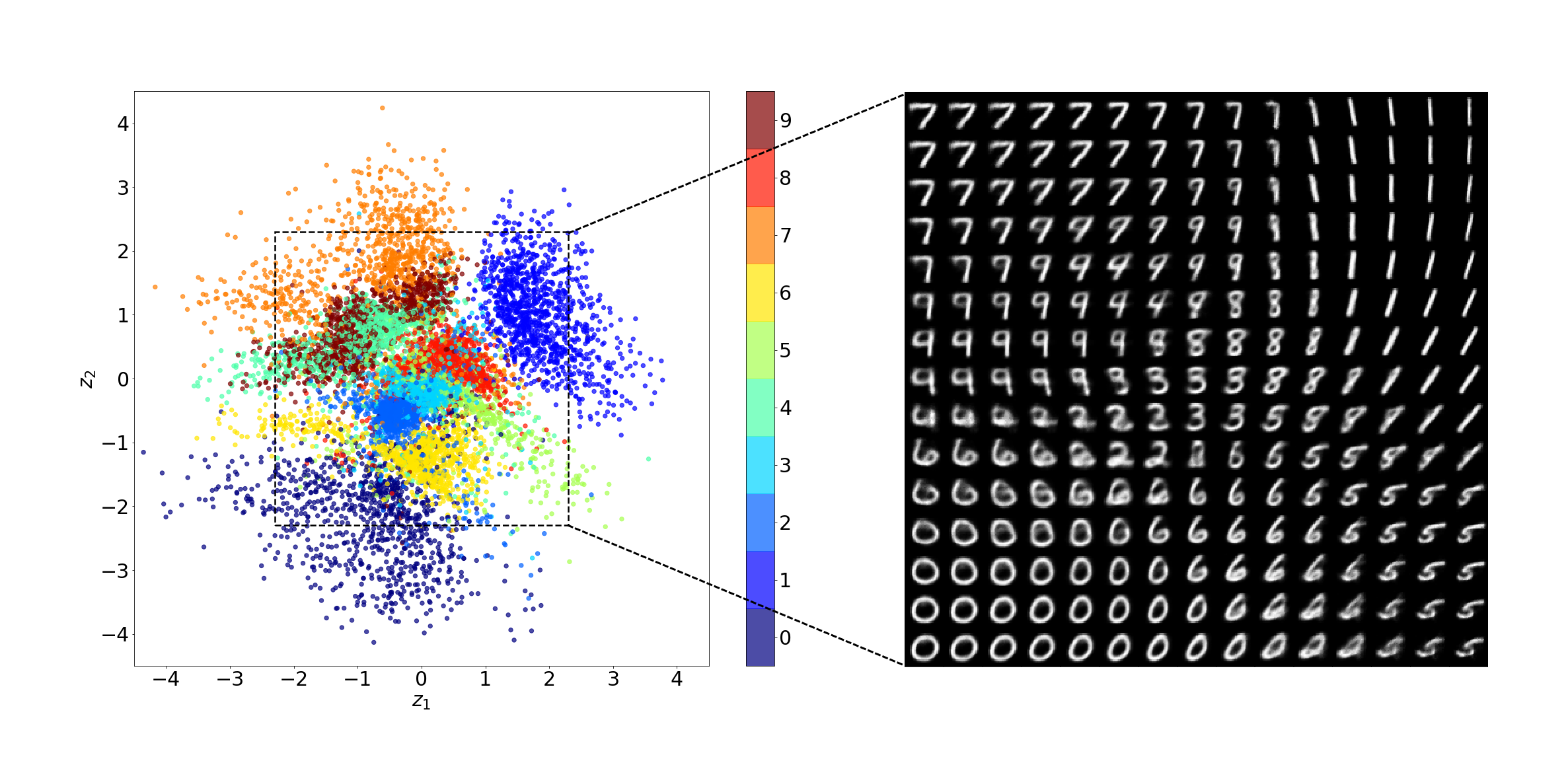
The model parameters \(\theta\) are learned through amortised variational EM, which requires learning an approximate posterior distribution \(q_{\phi}(\mathbf{z} \vert \mathbf{x}_i) \approx p_{\theta}(\mathbf{z} \vert \mathbf{x}_i)\). It is hoped that the learned \(q_{\phi}(\mathbf{z} \vert \mathbf{x})\) and \(p_{\theta}(\mathbf{x} \vert \mathbf{z})\) result in an informative latent representation of the data. For example, \(\{\mathbb{E}_{q_{\theta}(\mathbf{z} \vert \mathbf{x}_i)}[\mathbf{z}]\}_{i=1}^N\) cluster w.r.t. some discrete features or important factors of variation in the data, which often lie along the axes (up to some rotation or linear transformation):

The VAE is trained by minimising the evidence lower bound (ELBO) (Kingma and Welling, 2013), (Rezende et al., 2014)

where \(q_{\phi}(\mathbf{z}\vert\mathbf{x})\) and \(p_\theta(\mathbf{x}\vert\mathbf{z})\) are typically assumed to be diagonal Gaussians with their parameters defined as neural network functions of the conditioning variables, and \({p_\mathcal{D}(\mathbf{x})=\frac{1}{N}\sum_{i=1}^{N}\delta(\mathbf{x}-\mathbf{x}_i)}\) refers to the empirical distribution of the data \(\mathcal{D}\).

Variational Autoencoders as a constrained optimisation problem

First of all: why constrained optimisation?

The advantage of constrained optimisation is that it allows us to introduce conditions, which have to be fulfilled when optimising an objective function. In the context of VAEs, this can become especially important when it comes to complicated neural network architectures or hierarchical graphical models (Sonderby et al., 2016). The reason is: a low KL divergence is useless if the reconstruction fails. We therefore want to control the reconstruction quality.

To achieve this, Rezende and Viola (2018) proposed to formulate the learning problem as

\({\text{C}_\theta(\mathbf{x}, \mathbf{z})}\) is defined as the reconstruction error-related term in \({-\log p_\theta(\mathbf{x}\vert\mathbf{z})}\). Thus, requiring the average reconstruction error to be lower or equal than \(\kappa^2\). For example, in case of fitting continuous data, the reconstruction error is the quadratic loss \(\text{C}_\theta(\mathbf{x}, \mathbf{z})=\vert\vert \mathbf{x}- g_\theta (\mathbf{z})\vert\vert^2\) corresponding to a nonlinear conditional Gaussian likelihood model. The function \(g_\theta (\mathbf{z})\) is the decoder mapping the latent space into the data space.

The Lagrangian corresponding to the above optimisation problem is

and the learning is formulated as a saddle point optimisation of \(\mathcal{L}(\theta, \phi; \lambda)\) w.r.t. \((\theta, \phi)\) and \(\lambda\).

The main difference between \(\mathcal{L}(\theta, \phi; \lambda)\) and \(\mathcal{F}_\text{ELBO}(\theta, \phi)\) is the Lagrange multiplier \(\lambda\), which weights the inequality constraint. However, in general \(\mathcal{L}(\theta, \phi; \lambda)\) can only be guaranteed to be the ELBO if \(\lambda=1\), or in case of \(0\leq\lambda<1\), a scaled lower bound on the ELBO.

Note: in the classical constrained optimisation setting, constraints are not part of the objective function, and hence \(\theta\) would not be optimised. Otherwise, the convexity of the optimisation problem cannot be guaranteed. Let's go a few steps back to resolve this lack of clarity: within the VAE framework, it is a common practice to optimise (\(\theta, \phi\)) jointly. The original (EM) optimisation problem (e.g. (Neal and Hinton, 1998)), however, is formulated as

This perspective allows us to interpret the optimisation problem as a sequence of Lagrangians:

where \(\min_{\theta}\) and \({\max_{\lambda} \min_{\phi} \mathcal{L}(\theta, \phi; \lambda)}\) can be viewed as the corresponding steps of the original EM algorithm for training VAEs.

Hierarchical priors for learning informative latent representations

As the next step, we introduce an empirical Bayes prior within the above constrained optimisation setting. Referring to the argument in the beginning, such flexible priors avoid over-regularising the posterior distribution, and hence allow to incentivise the learning of informative latent representations.

It has been shown that the optimal empirical Bayes prior is the aggregated posterior distribution \(p^{\ast}(\mathbf{z}) = \mathbb{E}_{p_{\mathcal{D}}(\mathbf{x})}\big[q_{\phi}(\mathbf{z}\vert\mathbf{x})\big]\) (Tomczak and Welling, 2018). In order to express \(p^{\ast}(\mathbf{z})\), we use a continuous mixture/hierarchical model

and learn the parameters by applying an importance-weighted lower bound (Burda et al., 2015) on

This introduces a new optimisation objective

where \(p(\mathbf{\zeta})\) is a standard normal distribution and \(K\) the number of importance weights. We refer to this approach as variational hierarchical prior (VHP). As a result, we arrive at the Lagrangian

The constrained optimisation problem is formulated as

which leads to the following double-loop method:

• in the outer loop we update the upper bound (empirical Bayes) w.r.t. \((\Theta, \Phi)\);
• in the inner loop we solve the original constrained optimisation problem w.r.t. \({(\theta, \lambda, \phi)}\).

The Lagrange multiplier \(\lambda\) is updated by a quasi-gradient ascent. The update step is defined so that it finishes at \(\lambda = 1\), in order to optimise the ELBO at the end of the training. For more details regarding the \(\lambda\) update scheme and the optimisation algorithm, we would like to refer to our paper which is published at NeurIPS 2019.

Our proposed method, which is a combination of an ELBO-like Lagrangian and an importance-weighted bound on the optimal empirical Bayes log-prior distribution, can be interpreted as follows:

• the posterior of the first stochastic layer \(q_\phi(\mathbf{z}|\mathbf{x})\) can learn an informative latent representation due to the flexible prior;
• in order to express the flexible prior, we use a hierarchical mode and learn the parameters by applying an importance-weighted lower bound on \(\mathbb{E}_{p^{\ast}(\mathbf{z})} \big[\log p(\mathbf{z})\big]\).

Despite a diagonal Gaussian \(q_\Phi(\mathbf{\zeta}\vert \mathbf{z})\), the importance weighting allows to learn a precise conditional \(p_\Theta(\mathbf{z}\vert\mathbf{\zeta})\) from the standard normal distribution \(p(\mathbf{\zeta})\) to the aggregated posterior \(\mathbb{E}_{p_{\mathcal{D}}(\mathbf{x})}[q_{\phi}(\mathbf{z}\vert\mathbf{x})]\) (Cremer et al., 2017). Alternatively, one could use, for example, normalising flows (Rezende and Mohamed, 2015). Otherwise, the hierarchical prior might be not expressive enough and the model could compensate that by regularising \(q_\phi(\mathbf{z}|\mathbf{x})\). This would result in a restricted latent representation.

Comparison to Variational Autoencoders with standard Normal priors

Our key reason to introduce hierarchical priors was to get an informative latent representation. But does it work? To verify the quality of the latent representations, we build on the manifold hypothesis (Rifai et al., 2011). The idea can be summarised by the following assumption: real-world data presented in high-dimensional spaces is likely to concentrate close to nonlinear sub-manifolds of much lower dimensionality. Following this hypothesis, the quality of latent representations can be evaluated by interpolating between data points along the learned data manifold in the latent space—and reconstructing this path to the observable space.

To verify the above assumption, we use a k-NN graph, which is built based on samples from the (learned) prior—hence, based on the learned latent representation—with edge weights that are Euclidean distances in the latent space between the related node pairs. To find the shortest path through the graph we use \(A^\star\), a classic search algorithm.

In the following, we compare our method (VHP-VAE) to IWAE (Burda et al., 2015) a state-of-the-art method within the VAE framework that uses a standard normal prior.

CMU Human Motion Data

First, let's have a look at the learned latent representation of five different human motions based on the CMU Graphics Lab Motion Capture Database. This dataset is especially well suited for visualisations since it is simple enough for a two-dimensional latent space.

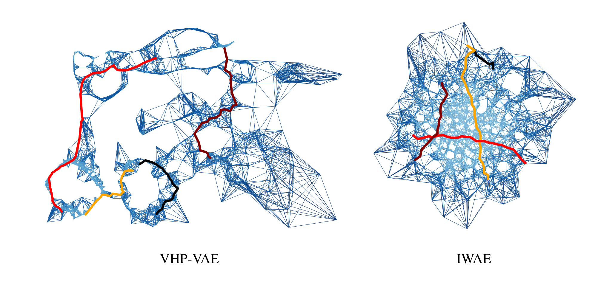
The k-NN graphs are built based on samples from the respective (learned) prior distributions. The bluescale indicates the edge weight and the coloured lines represent four human-movement interpolations between different poses. In case of the VHP-VAE, the latent representations of different movements are separated. By contrast, the IWAE cannot represent the different motions separately in the latent space since it is restricted by the standard normal prior. Reconstructing the above interpolations leads to the following human movements:

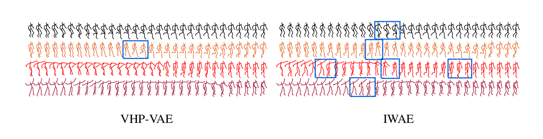
We marked discontinuities in the movements by blue boxes. Note that the VHP-VAE leads to smoother interpolations, whereas the IWAE interpolations show quite a few abrupt changes in the movements due to the missing structure in the latent space.

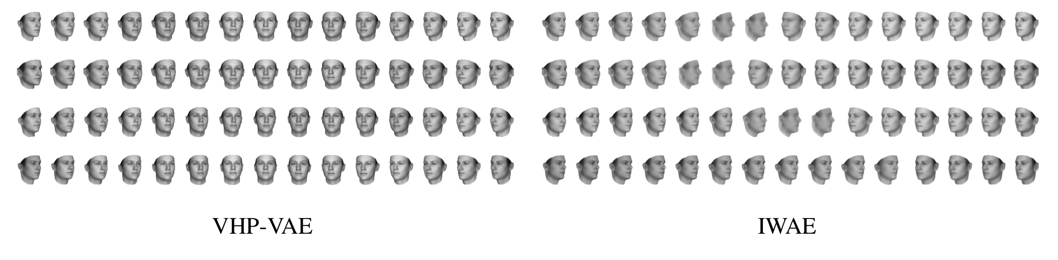
3D faces

How does the method scale to more complex data? To validate this, we show a small experiment on 3D faces (Paysan et al., 2009). In this case, the latent space is 32-dimensional:

Final words

In this blog post, we have seen that the learned hierarchical prior is indeed nontrivial, moreover, it is well-adapted to the latent representation, reflecting the topology of the encoded data manifold. The method provides informative latent representations and performs particularly well on data, where the relevant features change continuously.

This work was published (spotlight) at the Conference on Neural Information Processing Systems (NeurIPS), 2019 [preprint]

Bibliography

Alexander A Alemi, Ben Poole, Ian Fischer, Joshua V Dillon, Rif A Saurous, and Kevin Murphy. Fixing a broken ELBO. ICML, 2018. ↩
Samuel R. Bowman, Luke Vilnis, Oriol Vinyals, Andrew Dai, Rafal Jozefowicz, and Samy Bengio. Generating sentences from a continuous space. CoNLL, 2016. ↩
Yuri Burda, Roger B. Grosse, and Ruslan Salakhutdinov. Importance weighted autoencoders. CoRR, 2015. ↩ 1 2
Xi Chen, Diederik P. Kingma, Tim Salimans, Yan Duan, Prafulla Dhariwal, John Schulman, Ilya Sutskever, and Pieter Abbeel. Variational lossy autoencoder. CoRR, 2016. ↩
Chris Cremer, Quaid Morris, and David Duvenaud. Reinterpreting importance-weighted autoencoders. arXiv:1704.02916, 2017. ↩
Irina Higgins, Loic Matthey, Arka Pal, Christopher Burgess, Xavier Glorot, Matthew Botvinick, Shakir Mohamed, and Alexander Lerchner. Beta-VAE: Learning basic visual concepts with a constrained variational framework. ICLR, 2017. ↩
Diederik P. Kingma and Max Welling. Auto-encoding variational Bayes. CoRR, 2013. ↩ 1 2
Radford M Neal and Geoffrey E Hinton. A view of the em algorithm that justifies incremental, sparse, and other variants. In Learning in graphical models. 1998. ↩
P. Paysan, R. Knothe, B. Amberg, S. Romdhani, and T. Vetter. A 3d face model for pose and illumination invariant face recognition. AVSS, 2009. ↩
Danilo Jimenez Rezende and Shakir Mohamed. Variational inference with normalizing flows. ICML, 2015. ↩
Danilo Jimenez Rezende, Shakir Mohamed, and Daan Wierstra. Stochastic backpropagation and approximate inference in deep generative models. In Proceedings of the 31st International Conference on International Conference on Machine Learning - Volume 32, ICML'14, II–1278–II–1286. JMLR.org, 2014. URL: http://dl.acm.org/citation.cfm?id=3044805.3045035. ↩ 1 2
Danilo Jimenez Rezende and Fabio Viola. Taming VAEs. arXiv:1810.00597, 2018. ↩ 1 2
Salah Rifai, Yann N Dauphin, Pascal Vincent, Yoshua Bengio, and Xavier Muller. The manifold tangent classifier. NeurIPS, 2011. ↩
Casper Kaae Sønderby, Tapani Raiko, Lars Maaløe, Søren Kaae Sønderby, and Ole Winther. Ladder variational autoencoders. NeurIPS, 2016. ↩ 1 2
Jakub Tomczak and Max Welling. VAE with a VampPrior. AISTATS, 2018. ↩ 1 2