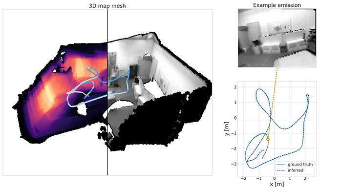
What if I told you that world models can scale to real 3D environments, can be fully probabilistic and can be inferred in real-time, all at once? Read on if you are interested, because we are about to lift the remaining runtime limitations from our last post.

This is the latest installment in a series focusing on spatial environments. So far in Part 1 we introduced a basic spatial state-space model, in Part 2 we scaled it to 3D, and in Part 3 we explored real-time tracking and planning in it.

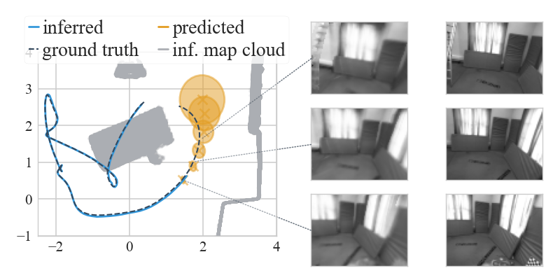
Probabilistic world models (e.g. Hafner et al. (2021), BeckerEhmck et al. (2020), Ha and Schmidhuber (2018)) are great. If we have such a model, we can predict possible futures for the agent and then robustly plan ahead under uncertainty. An example for that would be the orange rollout above. And if we do not have a model yet, we can invert the predictive assumptions to obtain it from data, with the help of Bayes.

This post is dedicated to the inference (or learning) of such models, and as the title suggests we will be dealing with spatial data exclusively. The challenge: how to do it in real-time, without giving up on expressivity and a fully-probabilistic treatment.

about spatial modelling

We believe an ideal spatial world model should faithfully predict the real world, it should be probabilistic, and it should be fast to obtain and to evaluate. The motivation is quite straightforward: expressive predictions for control, uncertainty to account for imperfections in the model and data, and speed for on-line use.

To comply, we have stuck to probabilistic state-space models since Part 1. In Part 2 we introduced differentiable rendering and 6-DoF states to our model, ensuring that inference and predictions scale to the real world. Yet, until now we had not reconciled the probabilistic and realistic prediction aspects with speed.

A problem we face is that differentiable rendering is expensive. This hinders commonplace stochastic optimisation methods like gradient descent because we need to render once per optimisation step. To add insult to injury, gradients through the renderer in a variational inference context will inevitably be noisy (i.e. when using the ELBO (Kingma and Welling, 2014)), which is a major drawback for convergence on a budget. Due to this limitation, in Part 3 we progressed towards real-time tracking and planning, but we had to rely on scenes learned off-line in advance.

Now it is time to get approximate posteriors over both the map and agent state in real-time.

filtering: divide and conquer

In the following we assume observations \(\,\obs_{1:T}\), agent states \(\,\state_{1:T}\) and controls \(\,\control_{1:T-1}\) form a Markovian state-space model (SSM), where a global map \(\,\map\) serves as the Bayesian parameters for a rendering emission model. In our notation, \(\,p(\cdot)\) will denote generative and true posterior distributions, and \(\,q(\cdot)\) will denote approximations. See the previous posts (Part 2, Part 3) for the details.

To achieve real-time inference, we change gears and target a filtering posterior instead of a smoothing one (Sarkka, 2013). Our motivation is in the paper, the short of it is that variational probabilistic smoothing under dense rendering is currently too expensive for us. The recursive update of a filter is easier to handle: we can concentrate computation better, and we can approximate some of it in closed form. Of course, this comes with a price which we accept for the sake of speed (see the end of this post). Let the history of observed data be \(\hist_t = \historyplus\), then we have:

The term \(\qfilter{t}{\map}\) is an approximate filter over the map, and \(\qfilter{t}{\state_t}\) is an approximate filter over the last agent state. They approximate the respective true posteriors \(\pfilter{t}{\map}\) and \(\pfilter{t}{\state_t}\). Note the difference to our inference from Part 2: we only estimate a posterior over the last state, not over the whole trajectory. This is motivated by the speed argument above and it is still enough for controlling the agent downstream.

Remember how we said rendering is expensive earlier? One way out is to design approximations that only render once per time step \(t\). This is much easier to do for a recursive filtering step than for a smoothing objective. We take advantage of this, and further combine well-established methods for closed-form updates into approximate filtering posteriors. We call the resulting method PRISM (Probabilistic Real-Time Inference in Spatial World Models). Here is a brief overview of what it boils down to in practice.

At every time step \(t\):

1. We point-estimate the agent’s pose \(\pose_t\), rendering once and involving geometry and dynamics.
2. We extend the pose \(\pose_t\) with a Gaussian covariance matrix through a Laplace approximation.
3. With the pose, we estimate the agent’s current velocity \(\vel_t\) in closed form via the dynamics model.
4. With the pose and the current observation \(\obs_t\), we update the map \(\map\) in closed form.

Mind you, here by "estimate/update" we mean inferring full probabilty distributions.

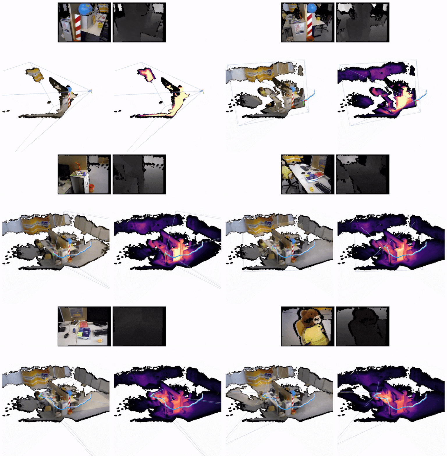
Here are two examples of how PRISM works in practice. The first is a drone trajectory (EuRoC), the video is in real-time and so is the inference:

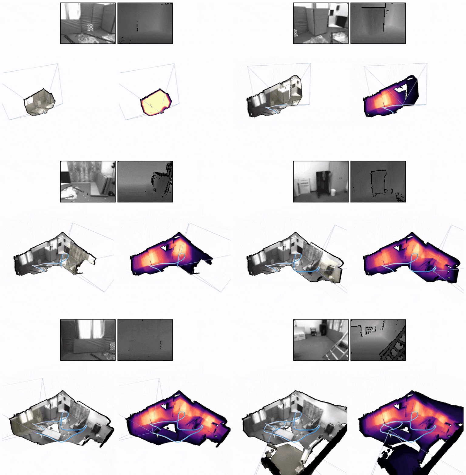
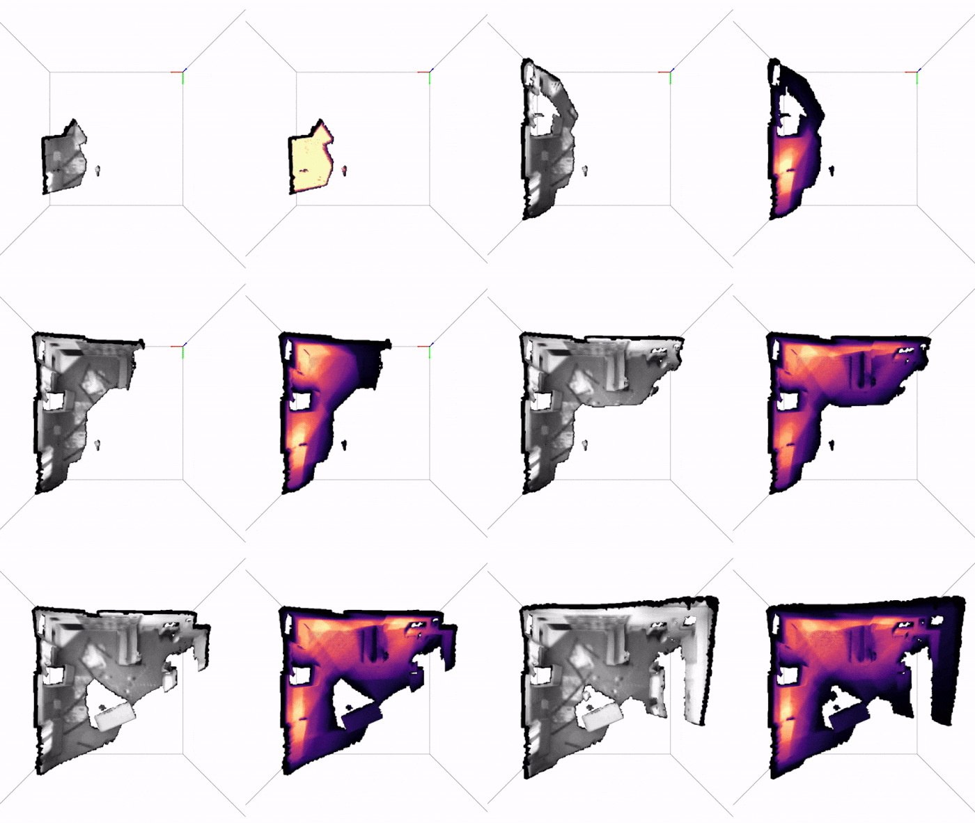
Note how we get live uncertainty for both the map (on the right) and for the states (which we do not display, for clarity of the visuals). Here is another example of applying PRISM to a handheld camera (TUM-RBGD):

Apropos, the derivation of both filters follows a classic recursive expression of the Bayes filter (Sarkka, 2013):

The math details are in the paper, and they lead to the practical implementation steps described above. To better see how these fit together, let us go over the final recursive update equations.

map updates

The final equation we derive for the map filtering update looks as follows:

Here, \(\qfilter{t-1}{\map}\) is the approximate Gaussian filter from the previous time step and \(\mapupdate\) represents an approximate Gaussian update over the map. The multiplication of both can be done in closed form, which is a conscious modelling choice for efficiency. This is a very fast way to obtain reasonable map uncertainty. It is significantly harder to ensure convergence of the map distribution on a budget when optimising the ELBO (Kingma and Welling, 2014) directly through the renderer.

The update \(\mapupdate\) is a function of the current observation and the current inferred pose of the agent. We identify SDF updates as compatible with our specific rendering assumptions and we interpret them probabilistically. In general, the map update can be redesigned for different map parameterisations or rendering assumptions.

state updates

State updates are slightly more involved, the end-product update rule we derive looks like this:

We make the assumption that states \(\state_t\) consist of a pose \(\pose_t\) and a velocity \(\vel_t\) (both linear and angular). First we track the agent pose as the maximum a posteriori (MAP) solution of the first two terms above:

Here, \(\poseprior\) is a one-step forward prediction distribution from the previous state filter, we obtain it with the help of the SSM's transition model. It makes the pose optimisation respect the agent dynamics. \(p(\obs_t \mid \hat \map, \pose_t)\) is the rendering emission (likelihood) model of the SSM. Just like in Part 3, we substitute it for point-to-plane ICP and photometric image alignment between a prediction rendered from the model and the current observation, we refer to the paper and the previous post for the details. This substitution allows us to render only once per time step. The overall pose optimisation looks like this:

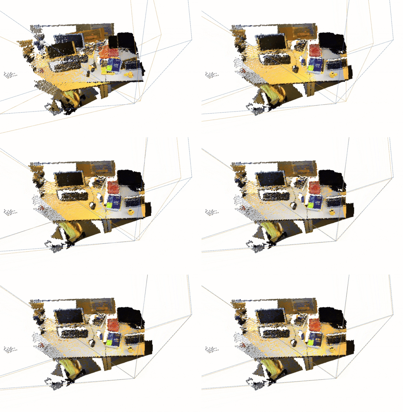
From there, we fit a Laplace approximation to the curvature of the objective to obtain pose uncertainty. And we finish off by linearising the dynamics and solving a linear Gaussian system to obtain a velocity estimate, involving the term \(\velcond\) from above (details are in the paper).

but filters can drift, right?

Absolutely, we see them only as a means to an end. Smoothing could be more optimal, but modern real-time SLAM smoothers assume sparsity, and generally rely on MAP point estimates of all variables. Since we want to capture dense maps with uncertainty in real-time, this is not a good fit for us. It is also worth noting that recursive closed-form updates for individual steps do not easily fit in with a smoother. In that sense, PRISM is an alternative solution for fully-probabilistic dense inference on a budget, trading off some potential accuracy for speed.

TL;DR

• Filtering is one viable way to obtain dense probabilistic spatial models in real-time.
• It works OK for moderately sized indoor scenes.
• Since stochastic gradient-descent optimisation through a renderer is expensive, we rely on one-shot closed-form updates where applicable instead.
• The inferred posterior distributions were designed to be sufficient for downstream control.

That's it, now you are familiar with our latest method in this series. As always, there are lots of improvements awaiting down the road, for example, uncertainty estimation is reasonable but still approximate, volumetric maps have a large memory footprint that we need to work around and we have not even touched the problem of dynamic objects in the scene.

That being said, PRISM was a much needed step forward for us. We can now start with autonomous acting on real hardware.

Stay tuned!

This work was published at the Conference on Robot Learning (CoRL), 2022 by Atanas Mirchev, Baris Kayalibay, Ahmed Agha, Patrick van der Smagt, Daniel Cremers and Justin Bayer. Here are the links: OpenReview, arXiv, supplementary material.

Bibliography

Philip Becker-Ehmck, Maximilian Karl, Jan Peters, and Patrick van der Smagt. Learning to fly via deep model-based reinforcement learning. 2020. URL: https://arxiv.org/abs/2003.08876, arXiv:2003.08876. ↩
David Ha and Jürgen Schmidhuber. World models. CoRR, 2018. URL: http://arxiv.org/abs/1803.10122, arXiv:1803.10122. ↩
Danijar Hafner, Timothy Lillicrap, Mohammad Norouzi, and Jimmy Ba. Mastering atari with discrete world models. 2021. arXiv:2010.02193. ↩
Diederik P Kingma and Max Welling. Auto-encoding variational Bayes. In Proceedings of the 2nd International Conference on Learning Representations (ICLR). 2014. ↩ 1 2
Simo Särkkä. Bayesian Filtering and Smoothing. Number 3. Cambridge University Press, USA, 2013. ISBN 1107619289. ↩ 1 2