Measuring the similarity between data points requires domain knowledge. But what if we don't have such knowledge?

We can compensate by relying on unsupervised methods such as latent-variable models, where similarity cq. distance is estimated in its compact, latent space. In that space one typically uses the Euclidean metric, but that ignores information about similarity of data stored in the decoder, as captured by the framework of Riemannian geometry. Alternatives—such as approximating the geodesic—are often computationally inefficient, rendering the methods impractical.

As we published at ICML in (Chen et al., 2020), we propose an extension to the framework of variational auto-encoders which allows learning flat latent manifolds, where the Euclidean metric is a proxy for the similarity between data points. This is achieved by defining the latent space as a Riemannian manifold and by regularising the metric tensor to be a scaled identity matrix. Additionally, we replace the compact prior typically used in variational auto-encoders with a recently presented, more expressive hierarchical one—and formulate the learning problem as a constrained optimisation problem.

Background

The background of this work can be found in the previous posts:

• Learning Hierarchical Priors in VAEs
• Riemannian geometry for generative models

Learning Flat Latent Manifolds with VAEs

We aim to develop flat manifold variational auto-encoders. This class of VAEs defines the latent space as Riemannian manifold and regularises the Riemannian metric tensor to be a scaled identity matrix.

In this context, a flat manifold is a Riemannian manifold, which is isometric to the Euclidean space. To not compromise the expressiveness, we relax the compactness assumption and make use of a recently introduced hierarchical prior (VHP-VAE). As a consequence, the model can learn a latent representation in which the Euclidean metric can be a proxy for the similarity between data points. The distance metric is then efficiently computed.

Our model—the VHP-VAE—can learn a latent representation with the same topology as the data manifold. But it cannot guarantee that the (Euclidean) distance in latent space is a sufficient distance metric in relation to the observation space.

In this work, we aim to measure the distance/difference of observed data directly in the latent space by means of the Euclidean distance of the encodings.

The latent space of a VAE is defined as a Riemannian manifold. This approach allows for computing the observation-space length of a trajectory \({\gamma:[0, 1]\rightarrow\mathbb{R}^{N_{\mathbf{z}}}}\) in the latent space:

where \(\mathbf{G}\in \mathbb{R}^{N_\mathbf{z} \times N_\mathbf{z}}\) is the Riemannian metric tensor, and \(\dot{\gamma}(t)\) the time derivative. We define the observation-space distance as the shortest possible path

between two data points. The trajectory \({\gamma=\text{argmin}_\gamma L(\gamma)}\) that minimises \(L(\gamma)\) is referred to as the (minimising) geodesic. In the context of VAEs, \(\gamma\) is transformed by a continuous function \(f(\gamma(t))\)—the decoder—to the observation space. The metric tensor is defined as \(\mathbf{G}(\mathbf{z})=\mathbf{J}(\mathbf{z})^{T}\mathbf{J}(\mathbf{z})\), where \(\mathbf{J}\) is the Jacobian of the decoder, \(\mathbf{z} \in \mathbb{R}^{N_{z}}\) represents latent variables and \(\mathbf{x} \in \mathbb{R}^{N_{x}}\) the observable data.

To measure the observation-space distance directly in the latent space, distances in the observation space should be proportional to distances in the latent space:

where we use the Euclidean distance metric to express the latent-space distance from start to end point of path \(\gamma\). This requires that the Riemannian metric tensor is \(\mathbf{G}\propto\mathbf{I}\). As a consequence, the Euclidean distance in the latent space corresponds to the geodesic distance. We refer to a manifold with this property as flat manifold.

So here's the thing: To obtain a flat latent manifold, the model typically needs to learn complex latent representations of the data. We do so with our previous work, the VHP, published at NeurIPS in 2019. It is used as follows: (i) to enable our model to learn complex latent representations, we apply a flexible prior (VHP) which is learned by the model (empirical Bayes); and (ii)~we regularise the curvature of the decoder such that \(\mathbf{G}\propto\mathbf{I}\), where \(\mathbf{I}\) is the identity matrix.

We obtain the objective function of our flat manifold VAE (FMVAE) by using the known VHP loss to which a regularisation loss of the decoder is added:

So: \(\mathcal{L}_\text{VHP}\) is the loss of the VHP-VAE (our previous post has more details), \(\eta\) is a hyperparameter determining the influence of the regularisation, \(c\) the scaling factor, and \({p_\mathcal{D}(\mathbf{x})=\frac{1}{N}\sum_{i=1}^{N}\delta(\mathbf{x}-\mathbf{x}_i)}\) is the empirical distribution of the data \(\mathcal{D} = \{\mathbf{x_i}\}^N_{i=1}\). Mixup allows augmenting data by interpolating between two encoded data points \(\mathbf{z}_i\) and \(\mathbf{z}_j\):

where \(\alpha\) is sampled from a uniform distribution.

Inspired by batch normalisation, we define the squared scaling factor to be the mean over the batch samples and diagonal elements of \(\mathbf{G}\):

A constrained optimisation is then proposed to update the parameters of the model.

Visualisation of equidistances on 2D latent space

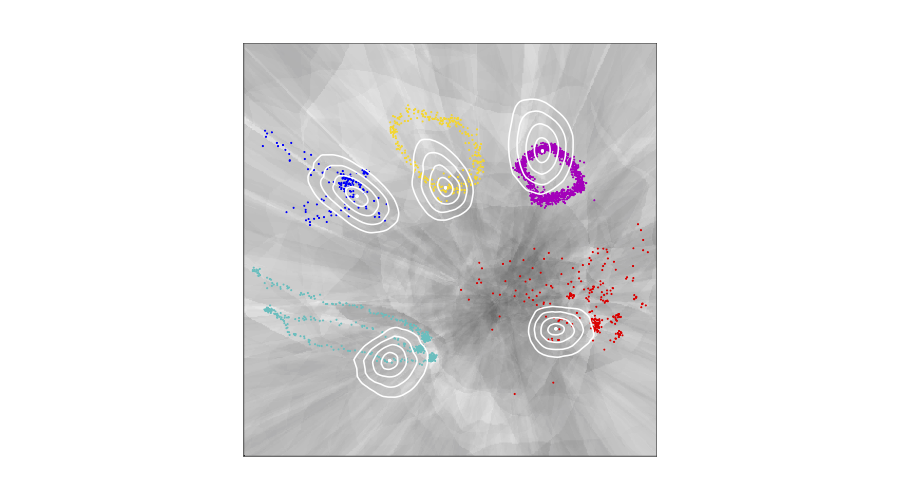
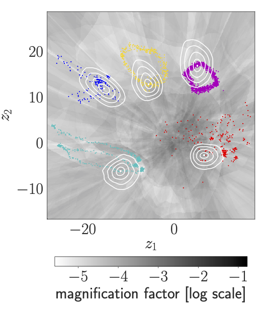
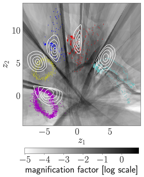
We visualise the Latent representation of CMU human motion data: the contour plots illustrate curves of equal observation-space distance to the respective encoded data point. The greyscale displays the magnification factor, \(\text{MF}(\mathbf{z})\). Note: round, homogeneous contour plots indicate that \({\mathbf{G}(\mathbf{z})\propto\mathbf{I}}\). In case of the VHP-FMVAE, jogging is a large-range movement compared with walking, so that jogging is reasonably distributed on a larger area in the latent space than walking. By contrast, in case of the VHP-VAE, the latent representation of walking is larger than the one of jogging. Additionally, geodesics are compared to the corresponding Euclidean interpolations. The Euclidean interpolations using the VHP-FMVAE are much closer to the geodesic.

VHP-FMVAE	VHP-VAE

VHP-FMVAE-SORT

We evaluate our approach on the MOT16 object-tracking database, which is a large-scale person re-identification data-set, containing both static and dynamic scenes from diverse cameras.

Our model is performed by replacing the appearance descriptor of supervised learning from DeepSORT with the latent space embedding from the various auto-encoders used, using the same size.

The numerical result shows that the performance of the proposed method is better than that of the model without Jacobian regularisation, and even close to the the performance of supervised learning (see more details in (Chen et al., 2020)). The following the an example of the performance of the proposed VHP-FMVAE-SORT.

Bibliography

Nutan Chen, Alexej Klushyn, Francesco Ferroni, Justin Bayer, and Patrick van der Smagt. Learning flat manifold of VAEs. In International Conference on Machine Learning (ICML). 2020. URL: https://arxiv.org/abs/2002.04881. ↩ 1 2