Continual Learning with Bayesian Neural Networks for Non-Stationary Data
Adapting to changing environments
Introduction
Continual learning (CL), also referred to as lifelong learning, is typically described informally by the following set of desiderata for computational systems: the system should (i) learn incrementally from a data stream, (ii) exhibit information transfer forward and backward in time, (iii) avoid catastrophic forgetting of previous data, and (iv) adapt to changes in the data distribution.
The necessity to adapt to non-stationary data is often not reconcilable with the goal of preventing forgetting. In the recent literature on continual learning, the latter has received significantly more attention. However, if the data distribution changes over time, old data may be "outdated" and can even deteriorate learning if the drift in the data distribution is neglected.
This blog post summarises our paper published at ICLR 2020, where we developed an approximate Bayesian approach for training Bayesian neural networks (BNN) incrementally with non-stationary streaming data.
Background: Online variational Bayes with Memory
Consider a stream of datasets \(\{ \mathcal{D}_{t_{k}} \}_{k=1}^{K}\), where \(t_k\) are the time points at which datasets \(\mathcal{D}_{t_{k}}\) are observed. In online learning, we want to learn from these datasets one at a time. For now, we assume that these datasets are independent and identically distributed (i.i.d.).
The Bayesian approach to online learning is based on the recursive application of Bayes' rule (posterior inference):
As usual, exact inference (within a family of commonly used distributions) is intractable for nonlinear models such as neural networks, therefore, approximations are required. Online variational Bayes achieves this by projecting the posterior distribution at every time step \(t_k\) into a simpler family of distributions \(q_{\theta_{t_{k}}}(\mathbf{w})\) with parameters \(\theta\):
In this work we consider diagonal Gaussian distributions \(q_{\theta_k}(w)\).
Online approximate Bayesian inference methods inevitably suffer from an information loss due to the posterior approximation at each time step. An alternative approach to online learning is to store and update a representative dataset/generative model—and to use it as a memory—in order to improve inference. Memory-based online learning and Bayesian approximations can also be combined by taking the product of two factors
and update them sequentially as new data \(\mathcal{D}_{t_{k}}\) are observed. The factor \(p(\mathcal{M}_{t_{k}} | \mathbf{w}) = \prod_{m}^{M} \, p(\mathbf{m}_{t_{k}}^{(m)} | \mathbf{w})\) is the likelihood of a set of \(M = \vert \mathcal{M} \vert\) data points, which we refer to as running memory; and \(q_{\theta_{t_{k}}}(\mathbf{w})\) is a Gaussian distribution, which summarises the rest of the data \(\bar{\mathcal{D}}_{1:t_{k}} = \mathcal{D}_{1:t_{k}} \backslash \, \mathcal{M}_{t_{k}}\).
Improving memory-based online variational Bayes
In the previous section we have seen how the posterior distribution can be approximated sequentially by two factors, a simple density (Gaussian) and a memory of raw data. The next question is how to best select which data we should use for the memory and which should be projected into the Gaussian distribution.
Properties of the Gaussian variational approximation
There are two interesting properties of the Gaussian variational approximation that are important for our work. We will use these in the next section and answer the above question.
First, the Gaussian variational approximation factorises into a product of Gaussian terms corresponding to the prior and each likelihood term. This result can be obtained by setting the derivatives of the ELBO w.r.t. the distribution parameters at a local optimum to zero, and writing the resulting equations as a sum of terms:
Since the natural parameters are given by a sum, the corresponding Gaussian factorises. As a result, it can be written in the form \(q_{\theta}(\mathbf{w}) = {Z_q}^{-1} p_{0}(\mathbf{w}) \prod_{n} \mathbf{r}^{(n)}(\mathbf{w})\), where the factors \(\mathbf{r}^{(n)}(\mathbf{w}) \approx p(\mathbf{d}^{(n)} \vert \mathbf{w})\) are the respective Gaussian functions and \(Z_q\) is the normalisation constant.
The second property is that, based on the above factorisation, the ELBO can be written in a form of difference terms between exact likelihood and its respective Gaussian approximation:
Next, we will use both properties to define update rules for our running memory and the Gaussian distribution.
Memory and Gaussian update
We want to select data for our running memory and the Gaussian in a complementary fashion, minimising the information loss due to the approximation with a simple density. The central idea of our approach is to replace the likelihood terms that can be well approximated by a Gaussian distribution through their Gaussian proxies \(p(\mathbf{d}_{t_{k}} | \mathbf{w}) \approx \mathbf{r}_{t_{k}}(\mathbf{w}; \mathbf{d}_{t_{k}})\) resulting in \(q_{\theta_{t_{k}}}(\mathbf{w})\); and retain the data corresponding to the rest of the likelihood terms in the running memory. To achieve this, we build on the ELBO formulation with difference terms from the previous section. If we replace the exact likelihood of a data point by its Gaussian proxy, then the two terms in the ELBO will cancel. In our work, we propose to replace/approximate the likelihood of those data points for which it makes least difference to the ELBO.
We proceed as follows: We first approximate the posterior of all data points at time-step \(t_k\) (including the running memory \(\mathcal{M}_{t_{k-1}}\)) by a Gaussian variational distribution \(\tilde{q}_{\theta_{t_{k}}}(\mathbf{w})\). Using the factorisation property of the Gaussian variational distribution (from the previous section), we can now compute the Gaussian proxies. Finally, using the ELBO formulation with difference terms (from the previous section), we select the memory using the following score function:
This score function will select data points for which using the Gaussian proxies makes the most difference to the ELBO and thus should be kept in raw form (at the current time step).
Having selected the running memory, updating the Gaussian \(q_{\theta_{t_{k}}}(\mathbf{w})\) is straightforward. We can simply combine all Gaussian terms that have not been selected for the running memory, or, equivalently, remove their contributions from \(\tilde{q}_{\theta_{t_{k}}}(\mathbf{w})\):
Results for memory-based variational approximation
Let us first look at some qualitative results and visually inspect the data points selected by our decision rule.
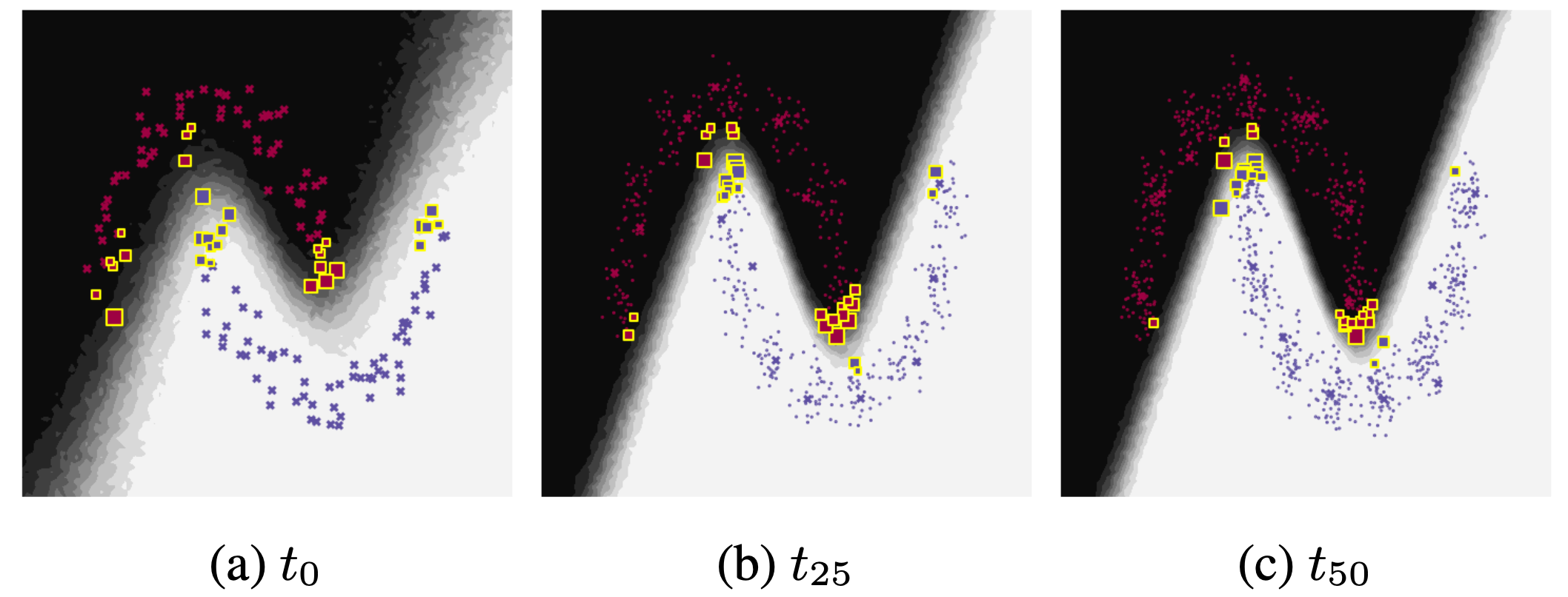
The figure shows the predictive distribution and data samples on a simple toy classification problem (two-moons dataset) at different time steps. Data from time step \(t_{k}\) and \(t_{\lt k}\) is visualised as large crosses and small dots, respectively, and data selected in the memory is marked with as yellow rectangles. As can be seen, our selection rule favours data points that are close to the decision boundary.
Variational Bayes with model adaptation
We have so far assumed data sets \(\mathcal{D}_{t_{k}}\) that arrive sequentially but being i.i.d., not only within each dataset but also between the different datasets. This assumption is made (often implicitly) for most recent continual learning algorithms and it may be reasonable in the typically considered multi-task scenarios where changes in the data distribution are algorithmic artifacts rather than natural phenomena. For example, in online multi-task or curriculum learning we want to learn a model of all tasks, but we may choose to learn the tasks incrementally in a certain order, where the ordering may be chosen random or according to some heuristic, e.g. first learning easier and then more difficult tasks.
However, the online i.i.d. assumption is wrong if the data distribution changes over time. For example, in online Variational Bayes (VB) the variance of the Gaussian posterior approximation shrinks at a rate of \(O(N)\), where \(N\) is the total number of data. Thus, learning will come to a halt as more and more data are observed; adaptation to changes in the data distribution is not possible.
In our work, we explored two alternative methods for adapting to changing data. In the first approach we impose Bayesian exponential forgetting between each tasks; in the second approach we implement the adaptation through a diffusion process applied to the neural network parameters. In the following, we present the approach using Bayesian forgetting.
Adaptation with Bayesian forgetting
Model adaptation through forgetting can be achieved by decaying the likelihood based on the temporal recency of the data and a Bayesian approach, involving a prior distribution and posterior inference, can be formulated as
where \(\tau\) is a time constant. The posterior of this new model involving decaying likelihood functions can be formulated sequentially, similarly to how we have shown in the beginning of this post:
This equation can be viewed as Bayes rule (for sequential inference, cf. beginning of this post) applied after a forgetting step. This forgetting step can be applied to both factors of our posterior approximation, the memory and the Gaussian distribution.
The effect of this forgetting operation, applied to the Gaussian distribution, is shown below.
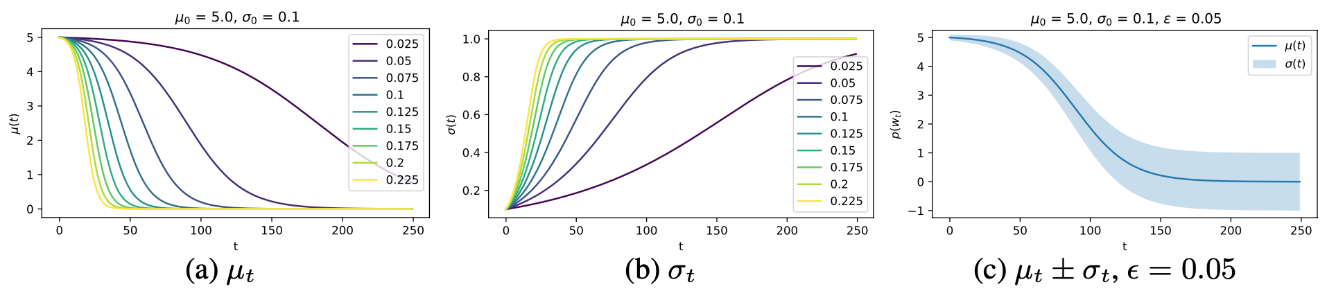
The plot shows the time evolution of distribution parameters when Bayesian Forgetting is applied, for different values of the forgetting parameter \(\epsilon\). The initial distribution (at \(t = 0\)) can be seen as the approximate posterior at some time-step \(t_k\). As can be seen, the distribution gradually reverts back to the prior distribution as \(t \rightarrow \infty\) (if no new data is observed in the meantime).
In the beginning of this section, we mentioned that the variance of the Gaussian in online Variational Bayes will shrink to zero as more data are observed and thus no adaptation is possible. We generated data from a simple logistic regression model for which the decision boundary rotates over time in a sinusoidal pattern. The approximate posterior of the model parameters (mean: line, std.dev: shaded) of an online inference algorithm (online Variational Bayes) and a model that uses Bayesian forgetting is shown below.
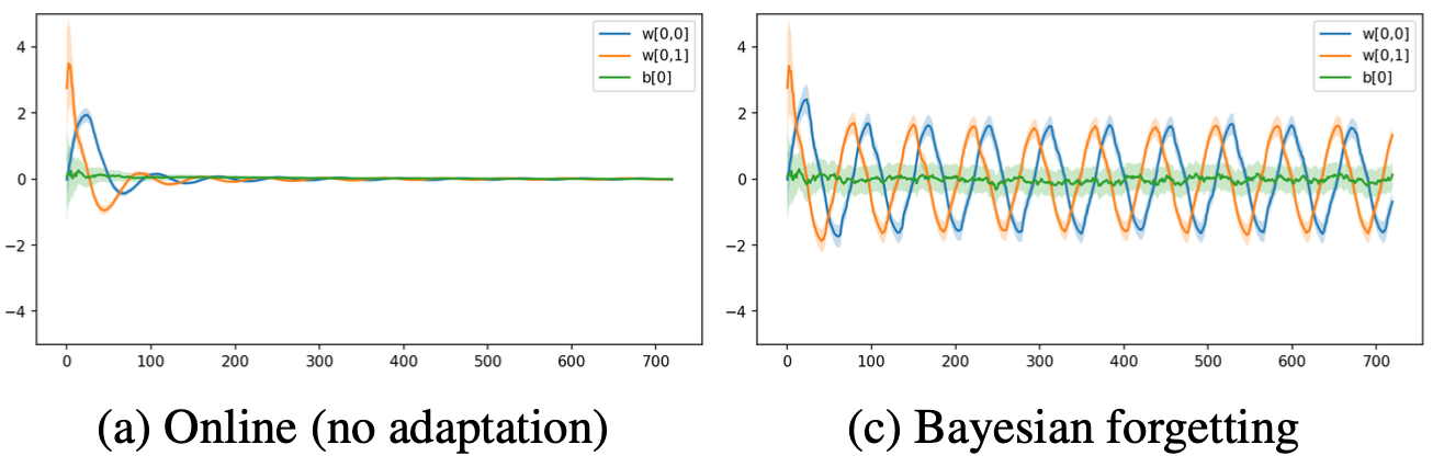
As can be seen, the online algorithm quickly stops learning and sets all parameters to zero which leads to a class distribution of 0.5 (maximally uncertain) everywhere. This makes sense since the data is equally distributed if we wait long enough and no classification is possible if we make the i.i.d. assumption. On the other hand, a model with Bayesian forgetting is able to adapt, since the likelihood of old data is decayed.
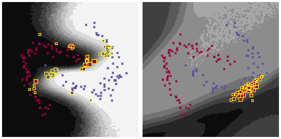
Similarly, we visualise the predictive distribution for a nonlinear toy classification problem (two-moons) where the data rotates.
Both models use online Variational Bayes (neural network with 2 hidden layers, 8 units, tanh) with memory (50 data points), with Bayesian forgetting (left) and without adaptation (right).
Let's further visualise OU process adaptation (without memory) and online Variational Bayes without adaptation and memory.

The model with OU process dynamics adapts immediately, much quicker than the model Bayesian forgetting. On the other hand, online VB is not able to "follow" the data distribution. It should be noted though, that online VB is not supposed to adapt since it assumes that all datasets \(\mathcal{D}_{t_{k}}\) are drawn from the same distribution; adaptation would thus be an artifact of the approximation algorithm rather than a designed and desired property.
Conclusion
In this post, we presented our work in which we addressed online inference for non-stationary streaming data using Bayesian neural networks. We have focused on posterior approximations consisting of a Gaussian distribution and a complementary running memory and we have used Variational Bayes to sequentially update the posteriors at each time step. We have proposed a novel update method, which treats both components as complementary, and two novel adaptation methods (in the context of Bayesian neural networks with non-stationary data), which gradually revert to the prior distribution if no new data are observed.
For more details and experimental results, please check out the paper.
This work was published at the International Conference on Learning Representations (ICLR), 2020. [openreview]