The holy grail of Bayesian inference is the posterior \(p(\mathbf z \mid \mathbf x)\) for a latent-variable model \(p(\mathbf{x, z})\).

We know it exists – which is a plus compared to the holy grail – but in almost all interesting cases it is equally elusive. Enter variational inference (VI). The goal of variational inference is to approximate the true posterior as best we can with a surrogate \(q(\mathbf z)\). In other words, we are trying to find a distribution that is tractable but as close as possible to the true posterior in the sense of the KL divergence,

A central pillar of research into VI is to improve the capacity of \(q\) to approximate the true posterior while keeping the distribution and the KL-optimisation tractable.

On Gaps

There are many reasons why the approximation may not be perfect. Researchers have started categorising these reasons. Such a taxonomy is useful because it helps us develop new approximation algorithms. This post will give you an overview of known inference suboptimalities, including a new one we recently discovered – the conditioning gap.

The reason we talk about gaps in this context is the connection between VI and the evidence lower bound (ELBO). The posterior KL which we seek to minimise is usually as intractable as the posterior itself, which is unsurprising considering that the posterior occurs in the divergence. Fortunately, there is a relatively easy way out. Since the evidence \(\ln p(\mathbf x)\) is constant in \(q\), it is easy to see that

By flipping the sign and adding a constant we – somewhat magically – end up with a tractable objective, the ELBO

The posterior KL divergence is now exactly the gap between evidence and ELBO, and consists of different parts.

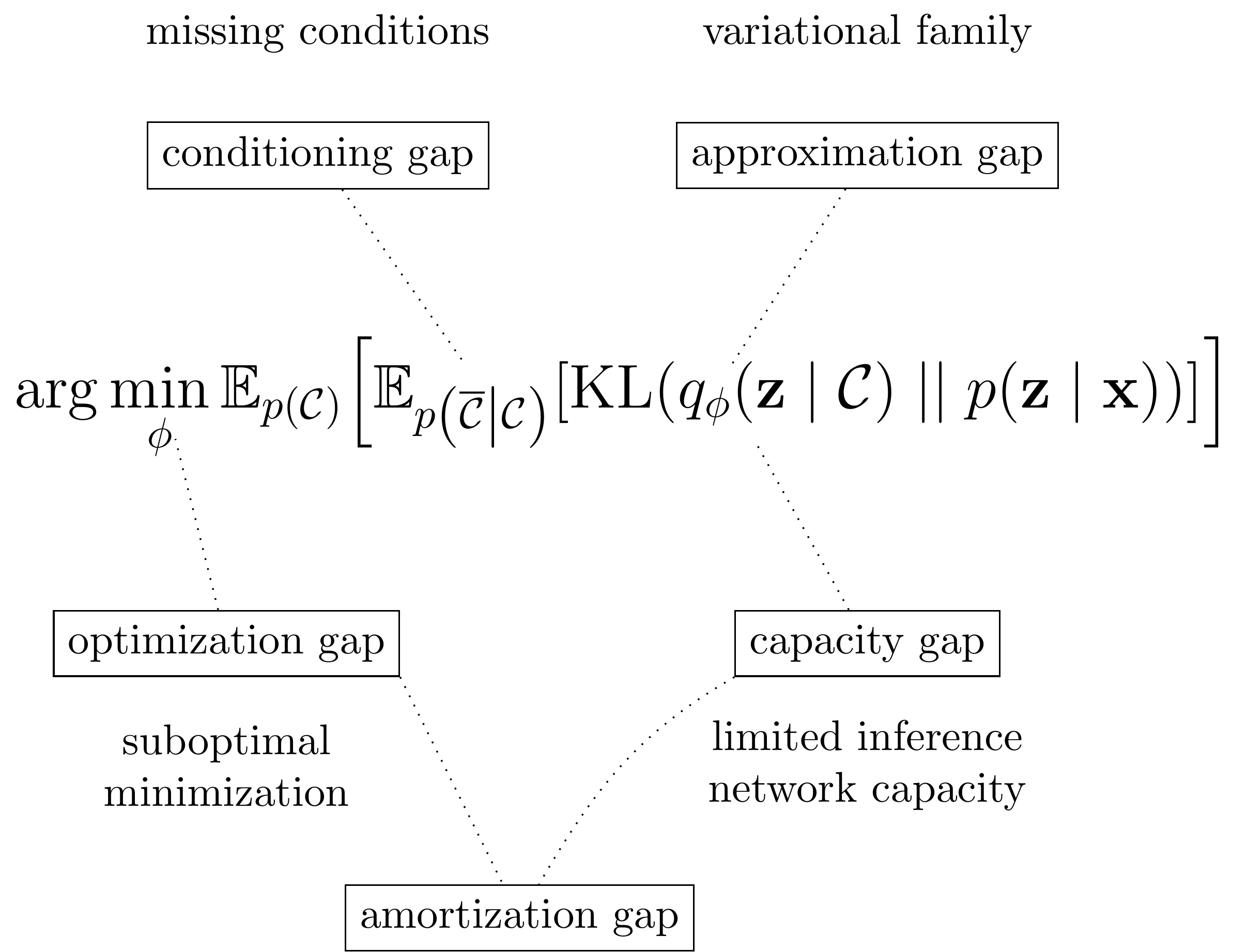
1) The Approximation Gap

The most straightforward of the gaps is the approximation gap. In the optimisation, an inconspicuous set \(\mathcal Q\) snuck in. This is the set of feasible variational approximations \(q\), the so-called variational family. Often, this is a family of tractable parametrised distributions, e.g., the set of Gaussian distributions, and we seek to find the optimal distribution parameters to approximate the true posterior within the variational family.

Usually, it is assumed that \(p(\mathbf z \mid \mathbf x) \notin Q\) – otherwise why even bother with approximations? From this, we can immediately tell that for all \(q\in\mathcal Q\)

The fact that the true posterior is not feasible – not a member of the variational family – introduces an irreducible gap: the approximation gap.

2) The Amortisation Gap

Variational auto-encoders (VAEs) shake up the VI formula a bit. Instead of an optimisation procedure, we use a neural network – the inference network – to determine \(q_{\phi}(\mathbf z \mid \mathbf x)\) for some observation \(\mathbf x\). (Note the slight change in notation from \(q(\mathbf z)\) to \(q_\phi(\mathbf z \mid \mathbf x)\) to reflect this more immediate functional relationship between \(\mathbf x\) and \(q\). The network parameters are denoted by \(\phi\).)

Using inference networks is considered amortising the cost of optimisation into a single forward pass, and this flavour of VI is hence called amortised variational inference. The inference network is trained by maximising the expected ELBO

The appeal of amortised inference is not improving VI, but speeding up VI. In fact, amortised VI generally returns worse approximations. This should not be surprising: the inference network still only returns a member of the variational family \(\mathcal Q\). It thus has the same constraints as VI in general. And unless we assume that the inference networks always finds the global optimum \(q^\star\) within \(\mathcal Q\) of the posterior KL divergence, its result will generally be a worse approximation than \(q^\star\), that is

This additional suboptimality is called the amortisation gap (Cremer et al., 2018). As long as the amortised approximation is good enough, the speed up of inference by neural networks can be considered worth the trade-off.

3) The Conditioning Gap

Which brings us to a new kind of gap that we discovered. Inference networks open a new design choice for approximate inference algorithms: which inputs to feed to the inference network. These need not be congruent with the true posterior. For instance, one could choose to only feed half the pixels of an image \(\mathbf x\).

What initially seems like a rather obscure choice turns out to be common practice in sequential variants of VAEs, including our very own deep variational Bayes filters (DVBFs). The true sequential posterior factorises as

Crucially, each of the factors contains future observations \(\mathbf x_{t:T}\), which we often do not have. After all, with DVBF (and many related methods), the idea is to learn a filter for downstream tasks like control. Filters by design should not access future observations. The initially obscure design choice becomes an almost natural, indeed the only possible choice in this setting.

As it turns out, its effects are much more severe than one might expect. To understand that – and to reduce notation clutter – we return to the non-sequential setting and split the observation \(\mathbf x\) into included conditions \(\mathcal C\) and excluded conditions \(\overline{\mathcal{C}}\), i.e., \(p(\mathbf z \mid \mathbf x) \equiv p(\mathbf z \mid \mathcal C, \overline{\mathcal{C}})\) etc.

The hope is that a partially-conditioned inference network \(q(\mathbf z \mid {\mathcal{C}})\) learns to approximate \(p(\mathbf z \mid \mathcal C)\) or \(p(\mathbf z \mid \mathcal C, \overline{\mathcal{C}})\) reasonably well. Model names like deep variational Bayes filters suggest as much. Unfortunately, this does not hold true as we found in our recent publication (Bayer et al., 2021).

The problem is that the inference network must now map all plausible data \(\mathbf x\) that share the same condition \(\mathcal C\) to the same amortised posterior \(q(\mathbf z \mid \mathcal C)\), even if they differ significantly in \(\overline{\mathcal{C}}\). We show that the mathematically optimal posterior \(q_{\mathcal C}(\mathbf z)\) is of the form

Superficially, this looks similar to the desired

Swapping the order of logarithm and expectation can drastically change the result though. The example in the figure below highlights this.

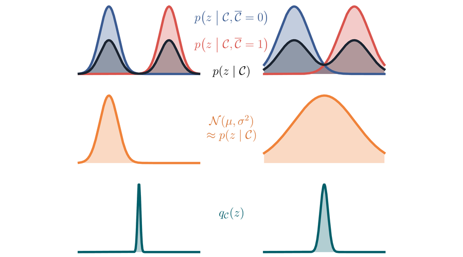
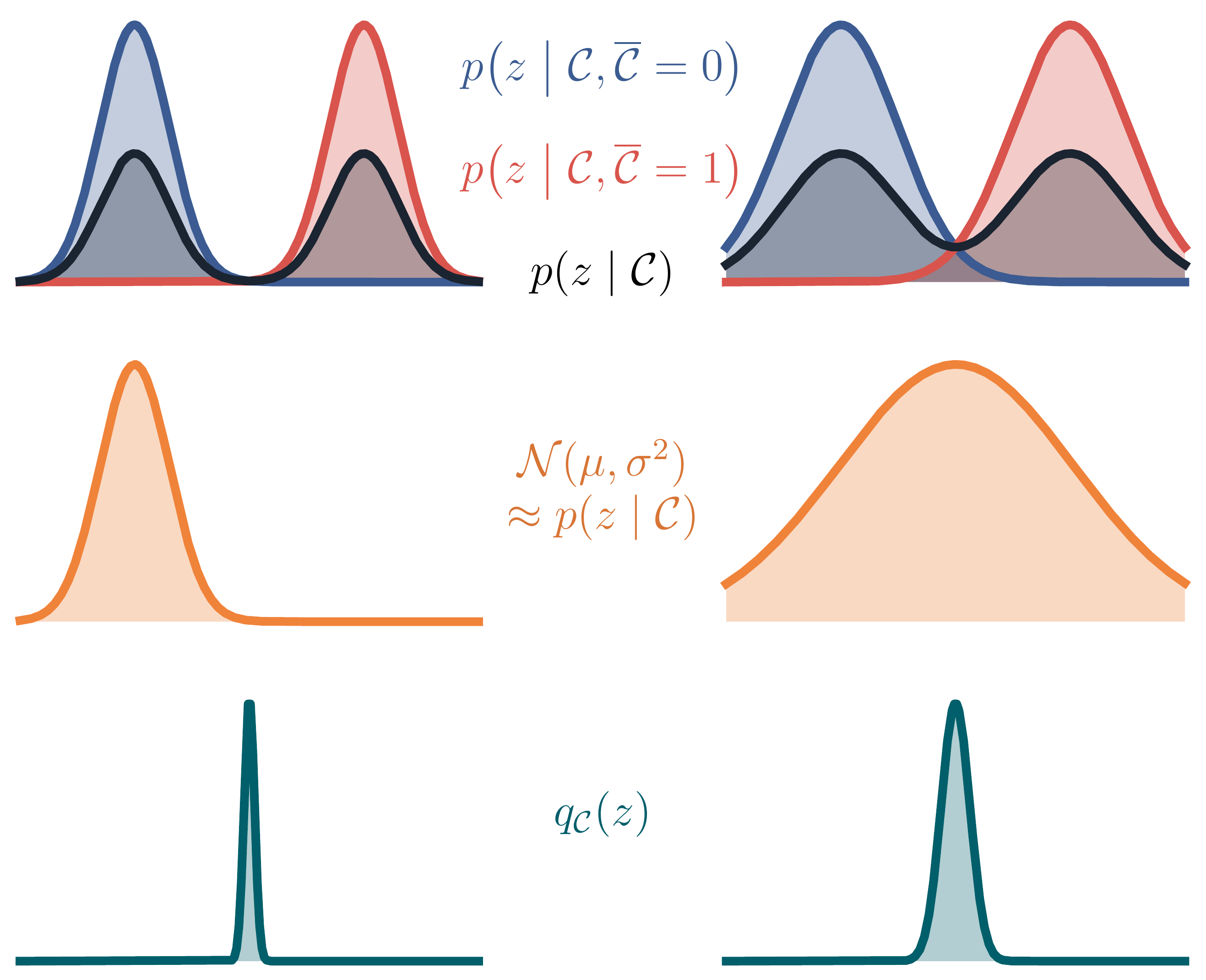
Here, we consider a simple model where the left-out condition \(\overline{\mathcal C}\) is a simple binary variable. In red and blue, we see the two true full posteriors depending on the value of \(\overline{\mathcal C}\). Left and right column show the same example but with different overlap of the two full posteriors. In black, we see the true partially-conditioned posterior, which is a mixture distrbution of the true fully-conditioned posteriors – in the absence of the missing bit, it maintains both beliefs.

The optimal Gaussian approximation of the mixture is depicted in orange. Given the restricted variational family, the approximation is reasonable in the sense that it covers the modes of the black mixture distribution.

Not so the optimal shared posterior \(q_{\mathcal C}(\mathbf z)\), depicted in teal. Due to the swapped order of expectation and logarithm, it is not a mixture distribution, but the (renormalised) product of the blue and the red curve. Unfortunately, this means that its mass concentrates where the two fully-conditioned posteriors can agree, which happens to be in regions where the true partially-conditioned posterior, the black curve) has little or no mass. Counterintuitively, the less the red and blue curves overlap, the more confident the shared posterior becomes. This behaviour is not desirable, and in particular very different from the behaviour of \(p(\mathbf z \mid \mathcal C)\).

We call this effect the conditioning gap. Our paper provides the details of this theoretical analysis, and also empirically verifies that it does play a role in various experiments.

Countering Inference Gaps

The point of putting a name to these various inference gaps is to subsequently devise strategies to counter them. To close this post, it is thus worth reflecting how to counter the three gaps we highlighted in this post.

1) The approximation gap is caused by a restrictive variational family \(\mathcal Q\). The obvious, if difficult, strategy is to extend the set of feasible distributions. Efforts to do so in the VAE literature have led to various flavours of normalising flows.

2) The amortisation gap on the other hand is caused by the inability of the inference network to map an observation \(\mathbf x\) to the optimal member of the variational family. This can have one of two reasons. One is that the inference network has limited capacity and cannot represent the optimisation procedure well. This is countered by increasing the capacity – more layers, wider layers, or better inductive biases in the network architecture. But even if we assumed sufficient capacity we may still encounter an amortisation gap. The reason is that we also need to find the optimal parameters of the inference network via optimisation, and we cannot guarantee perfect global optimisation.

Given that there are two orthogonal countermeasures for the amortisation gap, it may be worth splitting it yet again into an optimisation gap and a capacity gap, as depicted in the above overview of gaps. This is potentially interesting since the optimisation gap could be relevant to other VI methods such as stochastic VI.

3) Lastly, our newly found conditioning gap can be countered by carefully choosing the inference network inputs. In the simplest case, we can use all conditions as dictated by the true posterior — i.e., also use future observations. This need not be necessary, however. In the paper, we discuss scenarios where the conditioning gap is not as severe – examples include deterministic systems or systems with perfect state information.

Epilogue: Implications for Model-Based Reinforcement Learning

Hopefully this post has given you a good overview of the different gaps you should expect when using (amortised) variational inference. It is a curious topic in and of itself. In the limited scope of this post, we only discussed inference, but the implications of inference gaps and the conditioning gap in particular reach much further.

To understand why, we need to take one step back. VAEs are rarely used to just learn inference networks. Instead, we usually jointly learn the inference network along with the generative model \(p(\mathbf{x, z})\) with the intent of using the latter in downstream tasks. Our research shows that learning the generative model is affected by the conditiong gap that riddles the inference network. This has consequences for applications.

A prominent application of the past years is model-based reinforcement learning (MBRL). In the simplest terms, in MBRL we can make use of a sequential generative model and predict the future. In this simulator, we can safely optimise a policy. Flavours of the VAE have been used successfully. In follow-up work – which is still work in progress as of this writing – we examine whether the conditioning gap is relevant for MBRL. Spoiler: It is. For details, check out our recent workshop publication (Kayalibay et al., 2021).

This post is based on our recent ICLR publication (Bayer et al., 2021) and an overview of inference gaps in the author's recent PhD thesis submission. The latter is currently under review and will be provided here upon publication in the future. Until then the draft can be provided upon request.

Bibliography

Justin Bayer, Maximilian Soelch, Atanas Mirchev, Baris Kayalibay, and Patrick van der Smagt. Mind the Gap when Conditioning Amortised Inference in Sequential Latent-Variable Models. In 9th International Conference on Learning Representations, ICLR 2021. OpenReview.net, 2021. URL: https://openreview.net/forum?id=a2gqxKDvYys. ↩ 1 2
Chris Cremer, Xuechen Li, and David Duvenaud. Inference suboptimality in variational autoencoders. In Jennifer G. Dy and Andreas Krause, editors, Proceedings of the 35th International Conference on Machine Learning, ICML 2018, Stockholmsmässan, Stockholm, Sweden, July 10-15, 2018, volume 80 of Proceedings of Machine Learning Research, 1086–1094. PMLR, 2018. URL: http://proceedings.mlr.press/v80/cremer18a.html. ↩
Baris Kayalibay, Atanas Mirchev, Patrick van der Smagt, and Justin Bayer. Less Suboptimal Learning and Control in Variational POMDPs. In Self-Supervision for Reinforcement Learning Workshop - ICLR 2021. March 2021. URL: https://openreview.net/forum?id=oe4q7ZiXwkL. ↩